Decision Tree
Table of contents
Overview
Decision tree (DT) is a non-parametric supervised learning method.
It can be used for both classification and regression.
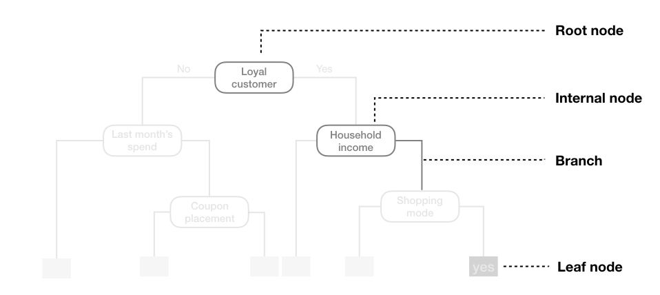
We start with the root node and do a recursive binary split on some feature condition (internal node) (such as $\text{feature} < \text{value}$) until we reach a leaf node, which represents a non-overlapping stratified region of the feature space.
Any multi-way split can be represented as a series of binary splits.
In classification, the output is a class label with the majority vote of the instances that fall in to the region of the terminal node (leaf).
In regression, the output is usually the mean of the instances in the terminal node.
Interpretation of Nodes
- The features split at each node represent the most informative feature for the current subset of data
- Features partitioned first are considered the most important factor in prediction
Advantages of DT
- Good interpretability
- Does not require much data preprocessing (such as scaling)
- Robust to outliers
- Able to handle both qualitative and quantitative features and labels
Disadvantages of DT
- Prone to overfitting
- You could literally have a tree that has a leaf for each data point, thus training error of 0
- “Pruning” unnecessary branches can help
- Feature value partitions can cause bias (see Caveat)
- Because tree nodes are decided by probability calculation, you may end up with completely different trees for “inherently” similar data when you slightly change the data
- This unstable nature can be mitigated by using random forests
- Not competitive in terms of accuracy
- Also mitigated by using random forests
Internal Node Selection
While decision trees are very intuitive, question remains:
How do we select which feature and where to split on in each layer of the tree?
In terms of regression, ideally we would like to minimize the residual sum of squares (RSS) across all the leaves:
\[\sum_{j=1}^{J} \sum_{i \in R_j} (y_i - \hat{y}_{R_j})^2\]where:
- $J$ is the number of leaves / regions
- $R_j$ is the $j$-th region
- $\hat{y}_{R_j}$ is the mean of the response values in region $R_j$ (prediction)
However, this is computationally infeasible.
Greedy Approach
We instead optimize on the binary RSS at each internal node:
$$ \underset{j, s}{\arg\min} \left[ \sum_{i: x_i \in R_1(j, s)} (y_i - \hat{y}_{R_1})^2 + \sum_{i: x_i \in R_2(j, s)} (y_i - \hat{y}_{R_2})^2 \right] $$
At each internal node, we consider all features $j$ and split points $s$:
\[R_1(j, s) = \{x_i \mid x_{ij} < s\} \quad \text{and} \quad R_2(j, s) = \{x_i \mid x_{ij} \geq s\}\]Then select the feature $j$ and split point $s$ that minimizes combined region RSS.
The minimizing $(j,s)$ is our internal node, and we repeat the process until a certain stopping criterion is met.
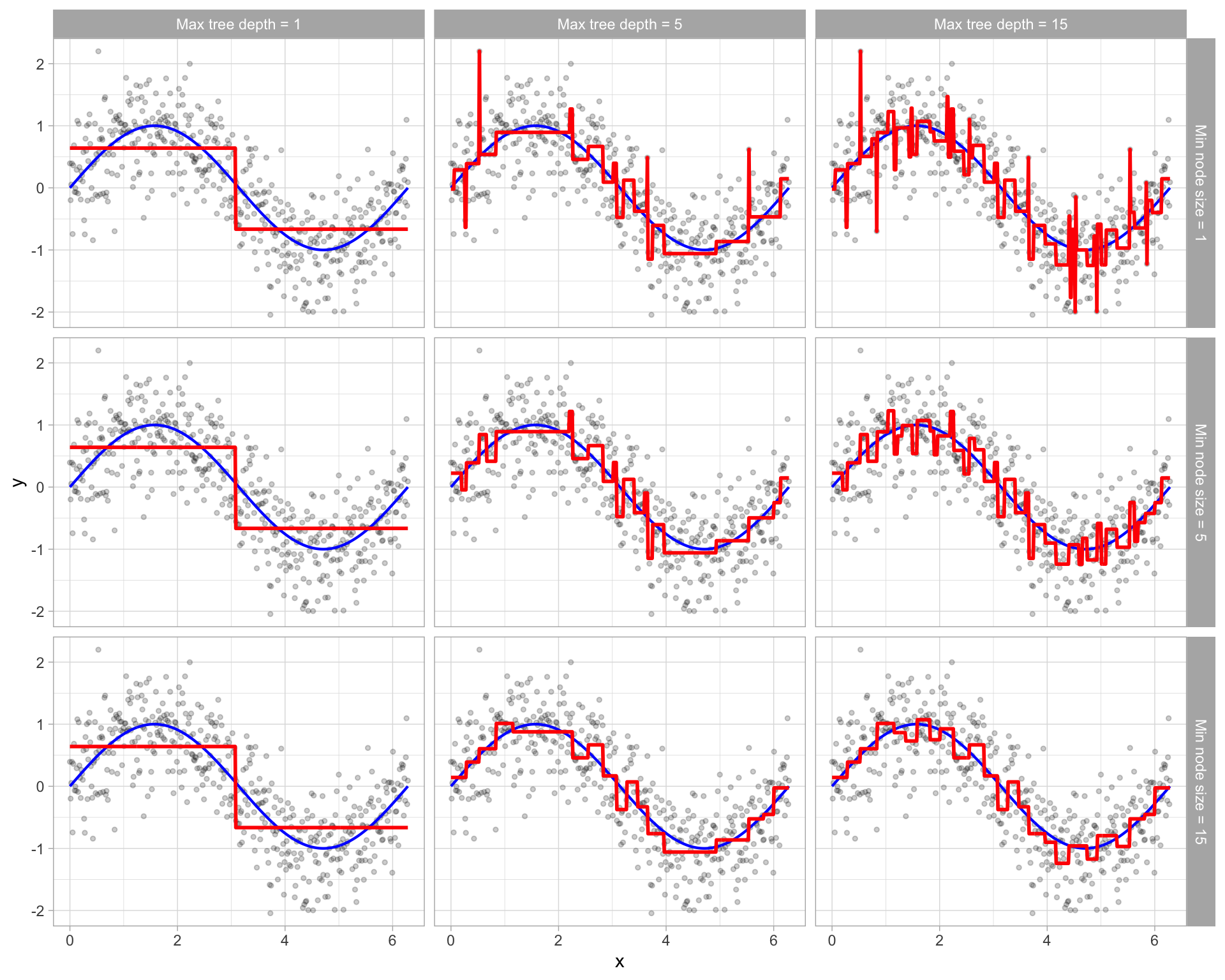
Stopping Criterion
Most common early stopping criteria are:
- Maximum depth
- Minimum samples per leaf
Pruning
We mentioned above that decision trees are prone to overfitting.
Pruning is the process of reducing a large tree after it is fully grown.
We do not want to prevent branching while the tree is growing: this leads to an overly short-sighted tree.
We denote the original large tree as $T_0$. We want to find a subtree $T \subset T_0$ that minimize the test error (via cross validation, etc.). However, we cannot possibly test all subtrees.
With cost complexity pruning or weakest link pruning we find a sequence of subtrees $T_\alpha$ indexed by $\alpha$.
In other words, for each tuning parameter $\alpha \geq 0$, we can find a subtree $T \subseteq T_0$ with the minimum penalized RSS:
$$ \sum_{m=1}^{|T|} \sum_{i: x_i \in R_m} (y_i - \hat{y}_{R_m})^2 + \alpha |T| $$
Which works in a similar way to regularization where the penalty is on the number of terminal nodes $|T|$.
Unlike the greedy approach used in buliding the original tree, we’re optimizing over the entire subtree.
With Cross-Validation
We can use cross-validation to find the best $\alpha$.
First shuffle and split the data into $K$ folds, and select a search range for $\alpha$.
For each $\alpha$:
For each fold k:
- Grow the tree $T_0$ to its maximum size with $K-1$ training folds
- Apply above formula to find the best subtree $T_\alpha$
- Calculate validation error on the $k$-th fold
Average the validation errors across all folds for each $\alpha$.
Find the minimizing $\alpha$ and use the corresponding subtree.
Internal Node Selection in Classification
In classification we need a different measure of error than RSS.
Since the class with the most training observations in a region becomes the predicted class for that region, we could think of using the misclassification rate:
\[\text{Error rate} = 1 - \max_k \hat{p}_{mk}\]Where $\hat{p}_{mk}$ is the proportion of training observations in the $m$-th region that belong to the $k$-th class.
However, misclassification rate is not sensitive enough for tree-growing purposes.
But during pruning, we use misclassification rate as a measure of error. The following measures are preferred during tree-growing becasue they are more sensitive to node purity than misclassification rate. However, they do not represent actual prediction accuracy.
The alternate options are as follows:
Gini Index
We could try to minimize the Gini index, a measure of impurity in a region:
$$ G = \sum_{k=1}^{K} \hat{p}_{mk} (1 - \hat{p}_{mk}) $$
Given a region $R_m$, if a single class $k$ dominates the region:
\[\hat{p}_{mk} \approx 1 \land \hat{p}_{mk'} \approx 0 \implies G \approx 0\]Small Gini index means the region is pure.
Entropy
Another measure of impurity or surprise in a region is entropy:
$$ D = -\sum_{k=1}^{K} \hat{p}_{mk} \log \hat{p}_{mk} $$
Small average surprise means the region is pure.
Numerically, Gini index and entropy are very similar.
Mutual Information
Or we could pick the feature that gives us the most information about the label.
For that we need an understanding of entropy and mutual information.
In short, entropy is the expected amount of information needed, and mutual information is the amount of information gain on one variable when we are given another, measured in terms of entropy.
Let $Y$ be the label and $X_i$ be the $i$-th feature.
For each feature $X_i$, we can calculate the mutual information between $X_i$ and $Y$.
Higher mutual information means that $X_i$ is more informative about $Y$, which is what we want.
\[\underset{X_i}{\arg\max} \; I(Y; X_i) = \underset{X_i}{\arg\max} \; H(Y) - H(Y \mid X_i)\]Caveat
One caveat is that mutual information is biased towards features with more partition.
For two features ID and gender, while there are many distinct values that ID can take on, gender only has so many.
So when you split on a feature with many distinct values (quantitative or not), we need to penalize by the number of splits and use a metric called information gain ratio, or just partition on a reasonable range.