Basic Probability Theory
Table of contents
Sample Spaces and Events
The sample space is the set of all possible outcomes of an experiment.
It is often denoted by $\Omega$.
Elements $\omega \in \Omega$ are called realizations or outcomes.
An event is a subset of the sample space.
Mutually Exclusive
Let $A_i$ be events. Then $A_i$ are mutually exclusive or disjoint if:
$$ A_i \cap A_j = \emptyset \quad \forall i \neq j $$
Disjoint events are not the same as independent events.
Partition
A partition of a sample space $\Omega$ is a set of mutually exclusive events whose union is $\Omega$:
$$ \bigcup_{i} A_i = \Omega $$
Probability
Probability is a function that maps an event to a real number: $P: \Omega \rightarrow \mathbb{R}$.
In general, we use the following notation for probability of an event $A$:
$$ P(A) $$
Interpretation of Probability
- Frequentist interpretation: The probability of an event is the limit of the relative frequency of the event as the number of trials goes to infinity.
- Bayesian interpretation: The probability of an event is the degree of belief.
Random Variable
Let $X$ be a random variable.
Probability of $X$ taking a value $x$ is denoted by:
$$ P(X = x) $$
Probability Distribution
Let $X$ be a random variable.
A probability distribution is a function that maps each value of $X$ to its probability.
In inferential statistics, we assume a certain probability distribution for the population. Then the samples become random variables that follow the same probability distribution.
Discrete Probability Distribution
The probability distribution of a discrete random variable $X$, is essentially the probability of each value of $X$.
Probability Mass Function
The probability mass function (PMF) of a discrete variable $X$ is denoted by:
$$ p_{X}(x) $$
This function maps each value of $X$ to its exact probability.
For discrete random variables, the PMF is the probability distribution.
$$ P(X = x) = p_{X}(x) $$
Continuous Probability Distribution
The probability distribution of a continuous random variable $X$, is the area under the curve of the probability density function (PDF) of $X$ for a given interval.
Probability Density Function
The probability density function (PDF) of a continuous variable $X$ is denoted by
$$ f_{X}(x) $$
The absolute probability of $X$ taking a specific value is zero, since there are infinitely many values that $X$ can take.
Therefore, the PDF of $X$ is not an absolute probability, but a relative probability per unit range.
Let $f_{X}(x)$ be the PDF of $X$. Then the probability that $X$ takes a value in the interval $[a, b]$ is:
$$ P(a \leq X \leq b) = \int_{a}^{b} f_{X}(x) dx $$
Cumulative Distribution Function
The cumulative distribution function (CDF) of a random variable $X$ is a non-decreasing function denoted by:
$$ F_{X}(x) = P(X \leq x) $$
CDF contains all the information about the probability distribution of $X$.
Therefore, for two random variables $X$ and $Y$, if their CDFs are the same, i.e.:
\[F_{X}(x) = F_{Y}(x) \quad \forall x \in \mathbb{R}\]then $X$ and $Y$ have the same probability distribution.
Properties of CDF
- $P(X = x) = F_{X}(x) - F_{X}(x^{-})$ where $x^{-}$ is the largest value less than $x$ (left-limit)
- $P(a < X \leq b) = F_{X}(b) - F_{X}(a)$
- $P(X > x) = 1 - F_{X}(x)$
Quantile Function
Let $X$ be a random variable with CDF $F_{X}(x)$.
The quantile function or inverse CDF of $X$ is:
$$ F_{X}^{-1}(q) = \inf \{ x : F_{X}(x) > q \} $$
where $q \in [0, 1]$.
Expected Value
The expected value of a quantitative random variable $X$ is denoted by:
$$ E(X) $$
It is a weighted average of the values of $X$, where the weights are the probabilities of each value.
Expected Value of Discrete Random Variable
Let $X$ be a discrete random variable. Then:
$$ E(X) = \sum_{x} x \cdot p_{X}(x) $$
Expected Value of Continuous Random Variable
Let $X$ be a continuous random variable. Then:
$$ E(X) = \int x \cdot f_{X}(x) dx $$
The range of the integral is the entire range of $X$.
Variance and Standard Deviation
Variance and standard deviation measures how much the values of a random variable $X$ are spread out from the expected value.
Standard deviation is the square root of variance.
Variance of Discrete Random Variable
Let $X$ be a discrete random variable. Then:
$$ V(X) = \sum_{x} (x - E(X))^{2} \cdot p_{X}(x) $$
Variance of Continuous Random Variable
Let $X$ be a continuous random variable. Then:
$$ V(X) = \int (x - E(X))^{2} \cdot f_{X}(x) dx $$
Some interesting properties of the variance/standard deviation:
- $V(X) \geq 0$
- $V(X) = 0$ if and only if $X$ is a constant
- Higher the value, higher the dispersion from the expected value
Joint Probability
Let $X$ and $Y$ be two random variables.
The joint probability of $X$ and $Y$ is denoted by:
$$ P(X, Y) $$
Also $P(X \cap Y)$, $P(XY)$.
Independent Random Variables
Two random variables $X$ and $Y$ are independent if:
$$ P(X, Y) = P(X) \cdot P(Y) $$
Conditional Probability
The conditional probability of $X$ given $Y$ is denoted by $P(X | Y)$.
$$ P(X | Y) = \frac{P(X, Y)}{P(Y)} $$
You could say that the sample space has changed from $\Omega$ to $Y$.
$P(X | Y) \neq P(Y | X)$ in general.
If $X$ and $Y$ are independent, then:
$$ P(X | Y) = P(X) $$
Common Probability Distributions
As described earlier, we assume a certain probability distribution for the population.
Each probability distribution has its own set of parameters.
These parameters determine the shape of the distribution.
Therefore, knowing the parameters is equivalent to understanding the population.
Below are some common probability distributions and their parameters.
Normal Distribution (Gaussian Distribution)
The normal distribution, also known as the Gaussian distribution, is a continuous probability distribution.
It is the most common distribution in statistics.
The normal distribution is characterized by two parameters:
- $\mu$: Mean (location of distribution)
- $\sigma$: Standard deviation (width of distribution)
The notation for the normal distribution is:
$$ X \sim N(\mu, \sigma^{2}) $$
The PDF of the normal distribution is:
$$ f_{X}(x) = \frac{1}{\sqrt{2 \pi \sigma^{2}}} e^{-\frac{(x - \mu)^{2}}{2 \sigma^{2}}} $$
Hard to see the exponent in the PDF?
$$ -\frac{(x - \mu)^{2}}{2 \sigma^{2}} $$
Characteristics of Normal Distribution
- Symmetric around the mean
- Mean, median, and mode are equal

- 68% of the values are approximately within $\mu \pm 1 \sigma$
- 95% of the values are approximately within $\mu \pm 2 \sigma$
- 99.7% of the values are approximately within $\mu \pm 3 \sigma$
Standard Normal Distribution
The normal distribution of $x$ against the probability density transformed into $z$ against the probability density is the standard normal distribution.
We can denote the standard normal distribution as:
$$ Z \sim N(0, 1) $$
Z-Score
Standardization or z-score normalization is the process of normalizing a dataset so that
$$ \begin{align*} \mu &= 0 \\ \sigma &= 1 \end{align*} $$
We do this by obtaining the standard score or z-score of each value by:
$$ z = \frac{x - \mu}{\sigma} $$
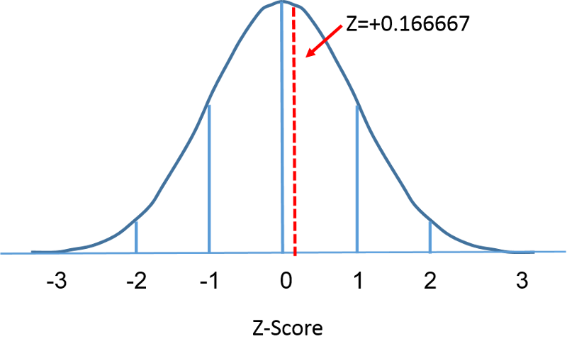
Z-score is essentially calculating how many $\sigma$ a value is away from the mean.
Higher the z-score, higher the value is from the mean.
Z-Score Table
Below is a part of the z-score table.
This table specifically, is for the left-tailed z-score. It shows the probability of a value being less than a certain z-score. Since the normal distribution is symmetric, the logic can be applied to the right-tailed z-score as well.
| Z | .00 | .01 | .02 | .03 | .04 | .05 | .06 | .07 | .08 | .09 |
|---|---|---|---|---|---|---|---|---|---|---|
| … | … | … | … | … | … | … | … | … | … | … |
| -2.1 | .01786 | .01743 | .01700 | .01659 | .01618 | .01578 | .01539 | .01500 | .01463 | .01426 |
| -2.0 | .02275 | .02222 | .02169 | .02118 | .02068 | .02018 | .01970 | .01923 | .01876 | .01831 |
| -1.9 | .02872 | .02807 | .02743 | .02680 | .02619 | .02559 | .02500 | .02442 | .02385 | .02330 |
| … | … | … | … | … | … | … | … | … | … | … |
Let’s use the z-score of 1.96 (absolute) as an example.
- Find the row with the z-score of $1.9$
- Find the column with the z-score of $0.06$
- You can see that the probability is $0.025$
Since the normal distribution is symmetric, we know that the probability of a value being greater than $1.96$ is also $0.025$.
Hence, the probability of a z-score falling outside of $\pm 1.96$ is $0.05$.
Others
To be added
Other common probability distributions include:
- Discrete Uniform distribution (discrete)
- Binomial distribution (discrete)
- Poisson distribution (discrete)
- Geometry distribution (discrete)
- Negative binomial distribution (discrete)
- Uniform distribution (continuous)
- Exponential distribution (continuous)
- etc.