Discriminant Analysis
One approach to classification was logistic regression.
Another approach is discriminant analysis.
Table of contents
Difference from Logistic Regression
Logistic regression:
- Does not assume any distribution for the features $X$.
- Is unstable when classes are well-separated.
- Harder to visualize for multinomial classification.
Distribution of Features
While logistic regression does not assume any distribution, discriminant analysis assumes some distribution for the features.
Most commonly, normal distribution.
Well-Separated Classes
When classes are well-separated, logistic regression does not converge.
The general idea is expressed in the following figure:
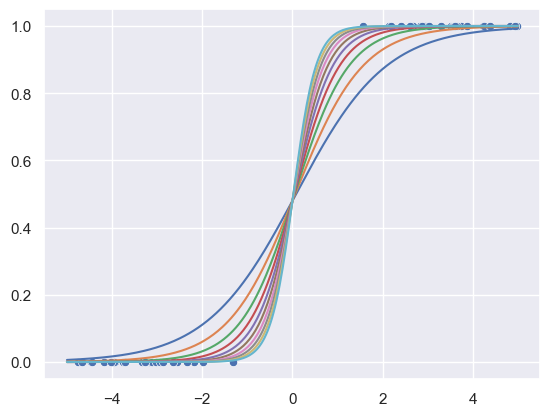
We see that there is no overlap between the two classes.
It is hard to determine which line is the best fit, which makes the model unstable.
Discriminant analysis benefits from well-separated classes.
In reality, classes are rarely well-separated. So logistic regression is still relevant to most problems.
Recap: Bayes’ Theorem
Classification aims to find the posterior:
$$ p_k(x) = P(Y = k \mid X = x) = \frac{P(X = x \mid Y = k) P(Y = k)} {\sum P(X = x \mid Y = l) P(Y = l)} $$
Notice that the marginal $P(X = x)$ is independent of the class $k$.
Remembering that optimal classfication is achieved by selecting the $k$ that maximizes the posterior, we can dismiss the denominator during our optimization (you would need it if you wanted the actual probability).
The product of the likelihood and prior ultimately determines the class of $X$, which gives us a convenient way to derive the discriminant score.
So now we need to find the likelihood and prior in the numerator.
Assumptions About the Likelihood
We usually denote the likelihood in each class as $f_k(x)$.
Discriminant analysis assumes some distribution for $X$ in a singe class $k$ (likelihood), which is usually a normal distribution (which results in LDA, QDA).
Single Feature
With a single feature $x$, the assumption is:
\[X \mid Y = k \sim N(\mu_k, \sigma_k^2)\]Then the likelihood is just the density function of the normal distribution:
$$ f_k(x) = P(X = x \mid Y = k) = \frac{1}{\sqrt{2\pi\sigma_k^2}} \exp\left(-\frac{(x - \mu_k)^2}{2\sigma_k^2}\right) $$
We can estimate this likelihood from the training data with sample mean and variance of the features in each class:
\[\hat{\mu}_k = \frac{1}{n_k} \sum_{i:y_i=k} x_i \quad\quad \hat{\sigma}^2_k = \frac{1}{n_k - 1} \sum_{i:y_i=k} (x_i - \hat{\mu}_k)^2\]Additional Assumptions about the Variance
Another assumption that can be made is that the variance of the features is the same for all classes:
$$ \sigma_k^2 = \sigma^2 $$
If you assume shared variance, we have a linear discriminant analysis (LDA).
If you do not, you have a quadratic discriminant analysis (QDA).
In LDA, our sample variance $\hat{\sigma}^2$ will be the pooled variance:
$$ \hat{\sigma}^2 = \frac{1}{n - K} \sum_{k=1}^K \sum_{i:y_i=k} (x_i - \hat{\mu}_k)^2 $$
Multivariate
With multiple features $X = (X_1, \dots, X_p)$, the assumption is that it follows a multivariate normal distribution:
\[X \mid Y = k \sim N(\mu_k, \Sigma_k)\]Then the likelihood is the density function of the multivariate normal distribution:
$$ f_k(x) = \frac{1}{\sqrt{(2\pi)^p \det(\Sigma_k)}} \exp\left(-\frac{1}{2} (x - \mu_k)^\top \Sigma_k^{-1} (x - \mu_k)\right) $$
Again, Additional Assumptions
Just like in the single feature case, you can assume that the covariance matrix is the same for all classes:
$$ \Sigma_k = \Sigma $$
Assuming this would result in LDA, while not assuming it would result in QDA.
Pooled Covariance
For multivariate normal distribution, we would estimate the covariance matrix $\Sigma$ using the pooled covariance:
\[\hat{\Sigma} = \frac{1}{n - K} \sum_{k=1}^K \sum_{i:y_i=k} (x_i - \hat{\mu}_k)(x_i - \hat{\mu}_k)^\top\]Estimating the Prior
We usually denote the prior of a class as $\pi_k$.
The prior of each class can also be estimated by the proportion of each class in the training data:
\[\hat{\pi}_k = \frac{n_k}{n} \approx P(Y = k)\]Obtaining the Posterior
So we obtain the posterior by plugging these estimates into Bayes’ theorem.
We usually rewrite the posterior as:
$$ P(Y = k \mid X = x) = \frac{\pi_k f_k(x)} {\sum_{l=1}^{K} \pi_l f_l(x)} $$
Linear and Quadratic DA
They both assume normal distribution for the features in each class.
Already mentioned above, but to recap:
The main difference between linear and quadratic discriminant analysis lies in the assumption about the variance of features in each class.
If we assume that the variance is the same for all classes:
$$ \sigma_k^2 = \sigma^2 \quad\quad \Sigma_k = \Sigma $$
the discriminant analysis becomes a linear classifier.
If we do not make this assumption, the discriminant analysis becomes a quadratic classifier.
Linear Discriminant Analysis (LDA)
We first start our estimate of the likelihood by assuming data in each class are normally distributed and have the same variance.
Plugging in the normal density function into the posterior would result in a super messy equation.
Discriminant Function (Discriminant Score) of LDA
If you wanted the actual probability of $X$ being in class $k$, you’d have to calculate the denominator.
But as we mentioned above, the marginal is independent of the class $k$.
If all you want is the class label of $X$ with the highest probability, you can ignore the denominator and try to maximize the numerator:
$$ p_k(x) \propto \pi_k f_k(x) $$
In addition, since log is a monotonic function, you can maximize the log of it instead:
\[\log(\pi_k) + \log f_k(x)\]Single Feature Discriminant Function
Fully expand the $\log$ and get rid of all the terms that are not dependent on $k$ to get the discriminant function of LDA:
$$ \delta_k(x) = x \cdot \frac{\mu_k}{\sigma^2} - \frac{\mu_k^2}{2\sigma^2} + \log(\pi_k) $$
Notice how the discriminant function is linear in $x$. If you did not assume $\sigma_k = \sigma$, you would have a quadratic discriminant function.
Then $x$ is assigned to the class $k$ that maximizes the discriminant score:
$$ k^\ast = \arg\max_k \delta_k(x) $$
Multivariate Discriminant Function
\[p_k(x) \propto \log(\pi_k) -\frac{1}{2} (x - \mu_k)^\top \Sigma^{-1} (x - \mu_k)\]Fully expand the right side and get rid of all the terms that do not depend on $k$ to get the discriminant function of LDA:
$$ \delta_k(x) = x^\top \Sigma^{-1} \mu_k - \frac{1}{2} \mu_k^\top \Sigma^{-1} \mu_k + \log(\pi_k) $$
Discrimant Functions to Probabilities
Discriminant scores can be converted to probabilities via the softmax function:
$$ P(Y = k \mid X = x) = \frac{\exp(\delta_k(x))}{\sum_{l=1}^{K} \exp(\delta_l(x))} $$
Discriminant Functions to Decision Boundaries
For graphing purposes, we could find the decision boundary between two classes $i$ and $j$.
The decision boundary is the set of points $\boldsymbol{x}$ where the discriminant scores are equal:
$$ \delta_i(\boldsymbol{x}) = \delta_j(\boldsymbol{x}) $$
Other Discriminant Analysis Methods
- Quadratic Discriminant Analysis (QDA):
- Relax the assumption $\Sigma_k = \Sigma$ from LDA.
- Naive Bayes:
- Assume that features are conditionally independent given the class.
- Useful when the number of features $p$ is large.
- Can be used for mixed feature types (quantitative and qualitative).