Encoding Categorical Variables
Categorical or qualitative variables are often non-numeric and must be encoded to be used in learning.
Table of contents
One-Hot Encoding
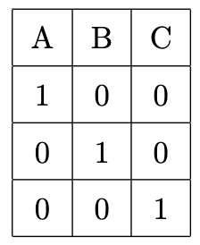
For a qualitative variable with $k$ groups, one-hot encoding introduces $k$ new binary variables.
For example, consider a variable $X$ with three groups: A, B, and C.
Dummy Variable Trap
There is one issue with one-hot encoding: the dummy variable trap.
If you look at the encoding, you can see that the third variable is redundant:
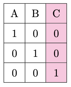
Because we could easily infer C by the encoding of A and B alone: 00.
This is a problem because now we have multicollinearity between our features.
Most one-hot encoding will have a parameter to automatically drop one of the dummy variables.
Dummy Encoding
Dummy encoding introduces one less binary variable than one-hot encoding, i.e., $k-1$ new binary variables.
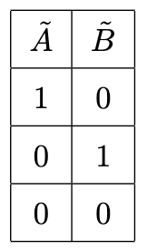
Each dummy represents
- $A \lor \neg A$
- $B \lor \neg B$,
and $\neg A \land \neg B \implies C$.
This avoids the dummy variable trap.
Baseline
With dummy encoding, one group is chosen as the baseline (in our example, C).
Say $X_1: A \lor \neg A$ and $X_2: B \lor \neg B$.
In simple linear regression:
\[Y = \beta_0 + \beta_1 X_1 + \beta_2 X_2 + \epsilon\]When the categorial variable is $C$ ($X_1 = 0$ and $X_2 = 0$),
\[Y = \beta_0 + \epsilon\]We are left with the baseline model.
Interpretation of Dummy Coefficients
In linear regression, the coefficients $\beta_i$ of quantitative variables are interpreted as such:
The average effect on $Y$ of a one-unit increase in $X_i$.
But how do we interpret the coefficients of dummy variables?
The effect is in comparison to the baseline.
So in our example above:
\[Y = \beta_0 + \beta_1 X_1 + \beta_2 X_2 + \epsilon\]where $X_1$ and $X_2$ are binary dummy variables for A and B, respectively:
- $\beta_0$ is the expected $Y$ when $X_1 = 0$ and $X_2 = 0$ (C)
- $\beta_1$ is the average effect on $Y$ when $X_1 = 1$ (A) compared to C
- $\beta_2$ is the average effect on $Y$ when $X_2 = 1$ (B) compared to C
It does not give you comparison between the effects of A and B.
Testing for Significance
After estimating $\beta_i$, we want to test whether each group is significantly different from the baseline.
Calculate the $t$-statistic for each $\beta_i$ as such:
$$ t = \frac{\hat{\beta}_i}{\text{SE}(\hat{\beta}_i)} $$
Remember that we are comparing each group to the baseline (is there a difference between A and C? B and C?).
You cannot compare the significance of arbitrary $\hat{\beta}_i$ and $\hat{\beta}_j$. For this, you must do a pairwise estimation for all groups.