Linear Regression
Table of contents
What is Linear Regression?
In statistical estimation, linear regression models the relationship between a dependent variable $y$ and one or more independent variables $x_i$ as a linear transformation of the independent variables plus some error/noise $\varepsilon$.
In general it models the relationship with the following equation:
- $y \in \mathbb{R}^{n \times 1}$ is the dependent variable
- $X \in \mathbb{R}^{n \times p}$ is the matrix of independent variables consisting of $n$ observations and $p$ features
- $\beta \in \mathbb{R}^{p \times 1}$ is the vector of coefficients
- $\varepsilon \in \mathbb{R}^{n \times 1}$ is the error term
To be more precise...
During actual estimation:
- $X$ is a matrix of dimension $(n, p+1)$ with the first column consisting of 1s (for the intercept term)
- $\beta$ is a vector of dimension $(p+1, 1)$ with the first element being the intercept term $\beta_0$
Just so that the matrix multiplication $X \beta$ produces:
$$ y_i = \beta_0 + \beta_1 x_{i1} + \beta_2 x_{i2} + \cdots + \beta_p x_{ip} + \varepsilon_i $$
$$ y = X \beta + \varepsilon $$
For a linear regression model, $\beta$ is the model parameter that we try to estimate.
Therefore, the prediction of the model is:
$$ \hat{y} = X \hat{\beta} $$
The model fitting process consists of estimating the parameter matrix $\beta$ such that the residual (difference between observed $y$ and predicted $\hat{y}$ value) is minimized.
The most common minimization method is the ordinary least squares (OLS) method.
Simple Linear Regression
Simple linear regression is a linear regression model with a single independent variable.
In other words, the number of features $p$ is equal to 1, so the feature matrix $X$ is a just a column vector.
Assuming each observation is independent of each other,
$$ y_i = \beta_0 + \beta_1 x_i + \varepsilon_i $$
where the error term has zero mean and constant variance:
\[\E(\varepsilon_i | X) = 0 \quad \land \quad \Var(\varepsilon_i | X) = \sigma^2\]Normality of the error term $\varepsilon | X \sim \mathcal{N}(0, \sigma^2)$ is not a requirement, but beneficial.
Entire process is equivalent to finding a best-fit line in a 2D graph.
Multiple Linear Regression
Multiple linear regression is a linear regression model with multiple independent variables.
$$ y_i = \beta_0 + \beta_1 x_{i1} + \beta_2 x_{i2} + \cdots + \beta_p x_{ip} + \varepsilon_i $$
Do not confuse this with multivariate linear regression, which is a linear regression model with multiple dependent variables.
Feature Selection
Polynomial Regression
Polynomial regression is actually just a special case of multiple linear regression.
It’s just that we transform the feature matrix to include polynomial terms.
Why is this linear?
What matters is the coefficients of the model, because they are the actual unknowns that we try to estimate while the features are collections of known values.
Although the features are in polynomial forms, the model itself is still a linear combination of the coefficients.
Interaction Terms
If some features are believed to be highly correlated, adding interaction terms to the 1-degree multiple linear model, which assumes independence of the features, can increase the model’s accuracy.
For example:
$$ Y = \beta_0 + \beta_1 X_1 + \beta_2 X_2 + \beta_3 \boldsymbol{X_1 X_2} + \epsilon $$
In this case,
- Positive $\hat{\beta}_3$: $X_1$ and $X_2$ amplify each other’s effect on $Y$
- Also called synergy
- Negative $\hat{\beta}_3$: $X_1$ and $X_2$ dampen each other’s effect on $Y$
Comparing the Effect to the Simpler Model
To see if the interaction term is needed,
- Compare the $R^2$ (explained variance) of models with and without the interaction term
- $R^2$ should be higher with interaction
- t-Test the significance of the interaction parameter
Hierarchical Principle
There is one caveat when using interaction terms:
If you include an interaction term in the model, you should also include the main effects.
Even if the main effects are tested to be insignificant, the interaction term can still be significant.
In such a case, the main effects should still be included in the model for the interaction term to be interpretable.
Non-Linear Terms
Maybe the relationship between the response and the feature is not linear.
In this case we can use transformed predictors to model the non-linear relationship, for example:
$$ Y = \beta_0 + \beta_1 X + \beta_2 \boldsymbol{X^2} + \epsilon $$
Adding this feature is valid because there is no linear dependency between $X$ and $X^2$.
Polynomial Feature Matrix
Amalgamating the above two concepts:
Single Feature
For a single feature $x$ and a polynomial degree of $d$,
$$ y_i = \beta_0 + \beta_1 x_{i} + \beta_2 x_{i}^2 + \cdots + \beta_d x_{i}^d + \varepsilon_i $$
Is still just our regular
\[y = X \beta + \varepsilon\]when we define the feature matrix $X$ as:
\[X = \begin{bmatrix} 1 & x_{1} & x_{1}^2 & \cdots & x_{1}^d \\ 1 & x_{2} & x_{2}^2 & \cdots & x_{2}^d \\ \vdots & \vdots & \vdots & \ddots & \vdots \\ 1 & x_{n} & x_{n}^2 & \cdots & x_{n}^d \end{bmatrix}\]This matrix is also called the Vandermonde matrix.
Two Features
For two features $x_1$ and $x_2$ and a polynomial degree of $2$,
$$ y_i = \beta_0 + \beta_1 x_{i1} + \beta_2 x_{i2} + \beta_3 x_{i1}^2 + \beta_4 x_{i2}^2 + \beta_5 x_{i1} x_{i2} + \varepsilon_i $$
so the feature matrix $X$ is:
\[X = \begin{bmatrix} 1 & x_{11} & x_{12} & x_{11}^2 & x_{12}^2 & x_{11} x_{12} \\ 1 & x_{21} & x_{22} & x_{21}^2 & x_{22}^2 & x_{21} x_{22} \\ \vdots & \vdots & \vdots & \vdots & \vdots & \vdots \\ 1 & x_{n1} & x_{n2} & x_{n1}^2 & x_{n2}^2 & x_{n1} x_{n2} \end{bmatrix}\]Only difference is that now joint polynomial terms are now included to model the interaction between the two features.
When we have $p$ features and a polynomial degree of $d$, the number of features becomes a combination of $p+1$ variables (including the intercept) selected $d$ at a time with repetition allowed. If you increase the complexity of the model too much, estimation becomes computationally expensive.
Also complex polynomial models are prone to overfitting.
When is it adequate to use linear regression?
For the linear model to be useful, typically the following checks should hold:
While some of the following conditions are intuitive, some of the not-so-obvious reasons come from the fact that they are required for parameter estimation to have a closed form solution, making estimation feasible or efficient (e.g. inverse of a matrix exists).
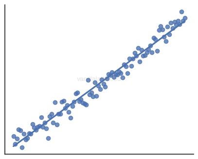
Linearity
The relationship between the feature and response variables, or the structure of the true model, should be linear.
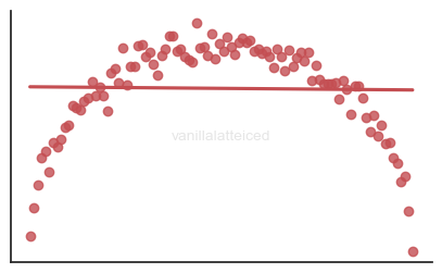
Quite obvious: you don’t want to fit an arch to a line:
No multicollinearity
The independent variables should not be correlated with each other.
If the value of one predictor is predetermined by the values of the other predictors, you have multicollinearity.
In other words, if you have an $n \times p$ feature matrix $X$, assuming $n > p$, the feature matrix should have full rank of $p$. Otherwise, you have multicollinearity between the features.
Multicollinearity can cause the following problems:
- Computationally expensive
- Increases unnecessary coefficients to be estimated
- The feature matrix becomes singular
- To be specific $X^\top X$ becomes singular
- Rank deficient matrices are not invertible, which is required for OLS to have a closed form solution
- Introduces confusion
- Harder to explain the effects of each predictor because they affect one another
Near-perfect collinearity
Maybe all features are linearly independent, in other words, they are not perfectly correlated. Then the closed-form solution for OLS exists.
However, even if the features are not perfectly correlated, high correlation makes the estimator unstable or high in variance, which could be an indication that the model is not suitable.
Zero conditional mean of the error
Linear regression is suitable if the unknown error term has zero conditional mean:
$$ \E(\varepsilon | X) = 0 $$
If you think about it, this assumption is essentially saying that the unknown error is negligible in determining the response.
This makes sense because if the error is so high that it dominates the response, there is no point in trying to model the relationship.
Check the residuals
Upon fitting the model, you should check the residuals to see if they are centered around zero.
Also, note the subtle difference between the error term and the residual.
Homoscedasticity of the error
Linear regression is suitable if the unknown error term has constant conditional variance:
$$ \Var(\varepsilon | X) = \sigma^2 $$
If you think about it, you want the data points to be within a certain boundary around the regression line for the model to be useful.
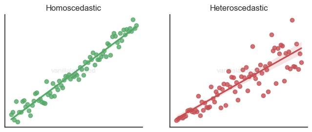
It’s not a bad model, but it can be an indication that a linear model may not be the most suitable structure.
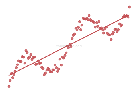
No autocorrelation of the residuals
Autocorrelation is the correlation with the lagged version of itself.
For linear regression to be suitable, there should be no autocorrelation.
In the figure below, there is a clear correlation between certain lagged periods:
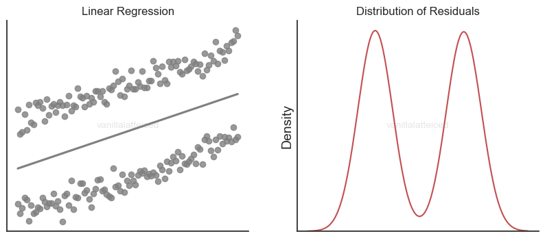
Normality of the error
If the linear regression model captures the relationship well enough, the residuals should be normally distributed.
For example, the following figure suggests maybe it wasn’t the best idea to use a single line to explain the samples:
Also having this condition brings additional benefits especially when using the OLS method for parameter estimation.
And most of the time, the OLS method is used for parameter estimation.
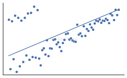
No outliers
Outliers are data points that are significantly different from the rest of the data.
If you know that these odd data points are truly outliers (in other words, they are not representative of the population, but only noise), then you can just remove them.
However, if these points are, although rare, representative of the population maybe due to some special features, then you should consider using a different model, because a linear regression model is not robust to outliers.
Modern ML libraries with linear regression models usually provide robust estimation methods that deweight outliers.