Regularization
Feature selection methods try to reduce variance and avoid overfitting by selecting a subset of predictors.
Regularization methods keep all predictors in the model, but reduce variance by shrinking the coefficients towards zero.
Table of contents
Shrinkage Methods
Compared to subset selection methods which select a subset of predictors, shrinkage methods or regularization methods keep all predictors, but try to shrink the coefficients towards zero.
Shrinking coefficients can significantly reduce the variance of the model.
Why does shrinkage reduce variance?
In regression, we try to estimate the coefficients $\beta$.
Shrinking the coefficients means we’re forcing our estimates to be closer to zero. Then we are introducing or adding bias to our estimates.
Recall back to the bias-variance tradeoff: Increasing bias reduces variance.
Regularized OLS is more rigid than regular OLS, hence the increased bias with reduced variance.
Ridge Regression
Examples are explained in the context of OLS, but it can be generalized to other regression models.
OLS’s objective is to minimize the residual sum of squares (RSS). Now we add an additional penalty term to the objective to control the magnitude of the coefficients:
$$ \min_{\beta} \left\{ \sum_{i=1}^{n} \left( y_i - \beta_0 - x_i^\top \beta \right)^2 + \lambda \lVert \beta \rVert_2^2 \right\} $$
Where the first part is just the RSS, and the second part is the shrinkage penalty and $\lambda \geq 0$ is the tuning parameter.
The intercept $\beta_0$ is usually not penalized, i.e. not included in the penalty term.
Shrinkage Penalty of Ridge
Shrinkage penalty of ridge relies on the squared L2-norm of the coefficient vector $\beta$:
\[\lVert \beta \rVert_2^2 = \sum_{j=1}^{p} \beta_j^2\]Some texts denote regularized coeffficents as:
$$ \hat{\beta}_{j,\lambda}^{R} $$
Tuning Parameter $\lambda$
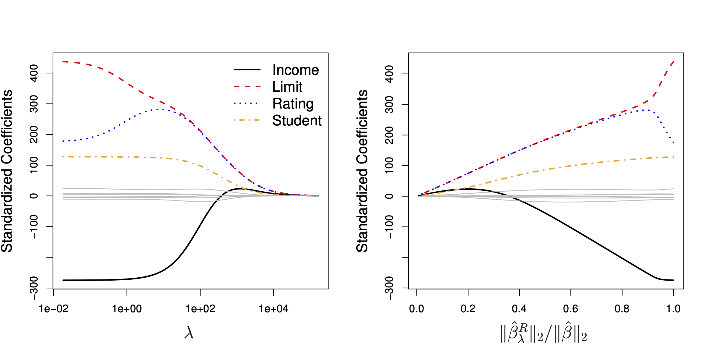
As $\lambda$ increases, we impose a larger penalty on the size of the coefficients, making the model more rigid and forces coefficients to shrink more towards zero:
\[\lambda \to \infty \implies \hat{\beta} \to \boldsymbol{0}\]Then we are left with the mean baseline model, or the intercept $\beta_0$.
In the figure above, notice how each predictor’s standardized (why?) coefficient converges towards zero as $\lambda$ increases.
However, in reality, we cannot make $\lambda$ infinitely large. So we never get a model with all coefficients exactly zero.
In addition, no coefficient $\beta_j$ becomes exactly zero in the ridge regression model. This is not the case for Lasso regression. See details in the later sections.
On the other hand, if $\lambda = 0$, there is no regularization and we get back OLS estimates.
Cross-Validation for $\lambda$

In the figure above:
- Pink: MSE
- Green: variance
- Black: bias squared
Regularization reduces variance and thus lowers the MSE up to a certain point (MSE is lowest near the middle, lower than when $\lambda = 0$).
However, as $\lambda$ increases further, the bias shoots up and MSE increases.
Therefore, we need to find the optimal $\lambda$.
We usually do this by cross-validation.
We would create folds and hold out a validation set, then for each $\lambda$ value, we perform cross-validation to estimate the test error and select the $\lambda$ that minimizes the test error.
Regularization is NOT Scale Equivariant
OLS estimates are scale equivariant. Multiplying a predictor by a constant $c$ only scales the coefficient by $1/c$, and thus:
\[c X_j \cdot \frac{\hat{\beta}_j}{c} = X_j \hat{\beta}_j\]Therefore, our predictions remain the same.
However, regularization methods, such as ridge and lasso, are not scale equivariant.
The unit of measurement of the predictors affects the coefficients, so whether you use 1 kilometer or 1000 meters matters.
Therefore, it is important to standardize the predictors before you apply regularization:
\[\tilde{X}_j = \frac{X_j}{\text{SD}(X_j)}\]Dividing each predictor by its sample standard deviation.
Lasso Regression
Again, examples are explained in the context of OLS, but it can be generalized to other regression models.
Unlike ridge regression, we use the L1-norm of the coefficient vector $\beta$ as the penalty term:
$$ \min_{\beta} \left\{ \sum_{i=1}^{n} \left( y_i - \beta_0 - x_i^\top \beta \right)^2 + \lambda \lVert \beta \rVert_1 \right\} $$
Again, with the tuning parameter $\lambda \geq 0$.
Shrinkage Penalty of Lasso
Shrinkage penalty of lasso relies on the L1-norm of the coefficient vector $\beta$:
\[\lVert \beta \rVert_1 = \sum_{j=1}^{p} \lvert \beta_j \rvert\]Similarly, some texts denote lasso regularized coeffficents as:
$$ \hat{\beta}_{j,\lambda}^{L} $$
Difference from Ridge
We mentioned above that no coefficient $\beta_j$ becomes exactly zero in the ridge regression model.
However, in the lasso regression model, coefficients can be exactly zero.
This has the effect of subset selection, because the influence of some predictors is completely removed from the model.
You should not be refitting the model with the non-zero predictors. Doing so would be a type of data leakage. The regularized coefficients are the final estimates.
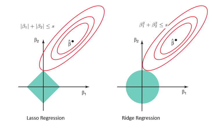
Our objective function is represented by the red level curves.
The first green diamond is our L1 constraint and the second is our L2 constraint:
\[\lVert \beta \rVert_1 \leq s \quad \text{and} \quad \lVert \beta \rVert_2^2 \leq t\]From lagrange multipliers, we know that the optimal minimum occurs when the level curves are tangent to the constraint region.
In Lasso, $\hat{\beta}$ has the potential to hit the upper corner of the constraint where (in this example) $\beta_1 = 0$.
However, that is not the case for Ridge.