Support Vector Machine
Table of contents
Basic concept of SVM
Support vector machine (SVM) is a supervised machine learning algorithm that can be used for both classification and regression.
Support Vector Classifier
Support vector classifier (SVC) is a binary classifier that finds the optimal hyperplane that separates the two classes.
Although SVC is inherently a binary classifier, it can be extended to multi-class classification (Lookup: one-vs-one, one-vs-rest, multiclass SVM).
Training data
- For $i = 1, \dots, n$,
- $\mathbf{x}_i \in \mathbb{R}^p$ is the $i$-th observation.
Do not confuse this notation with the $x_1$ and $x_2$ in the figure below. The $x_1$ and $x_2$ in the figure are notating the two hypothetical features just to illustrate the concept of SVC in a 2D space.
In our case, each $\mathbf{x}_i$ is a $p$-dimensional vector that represents the $p$ features of the $i$-th observation (so each colored dots in the figure below). - $y_i \in \{ -1, 1 \}$ is the (binary) class label of $x_i$.
- $\mathbf{x}_i \in \mathbb{R}^p$ is the $i$-th observation.
Hyperplane
A hyperplane is an affine subspace of dimension $p-1$ in $\mathbb{R}^p$.
A hyperplane in $\mathbb{R}^2$ is a line (1-dimensional subspace) and in $\mathbb{R}^3$ is a plane (2-dimensional subspace).
- We want to find the optimal hyperplane that separates the two classes.
- The optimal hyperplane is the one that maximizes the margin (Maximal Margin Classifier), which is the distance between the hyperplane and the closest observations.
We want to estimate a hyperplane defined by,
- $\mathbf{w} \in \mathbb{R}^p$ is the vector normal to the hyperplane.
- $b \in \mathbb{R}$ is the bias of the hyperplane.
- If $b = 0$, the hyperplane passes through the origin.
$$ \mathbf{w}^\top \mathbf{x} + b = 0 $$
Equation looks different
As in the figure above, sometimes people define the hyperplane with a negative bias term:
\[\mathbf{w}^\top \mathbf{x} - b = 0\]This is just a matter of notation and does not affect the estimation.

Support vectors
Support vectors are $\mathbf{x}_i$ that satisfy the following conditions:
$$ \begin{align*} \mathbf{w}^\top \mathbf{x}_i + b = 1 &\wedge y_i = 1 \\ \mathbf{w}^\top \mathbf{x}_i + b = -1 &\wedge y_i = -1 \end{align*} $$
More details
More generally, the support vectors are the observations that satisfy:
\[\begin{align*} \mathbf{w}^\top \mathbf{x}_i + b = a &\wedge y_i = 1 \\ \mathbf{w}^\top \mathbf{x}_i + b = -a &\wedge y_i = -1 \end{align*}\]However, with data normalization, we can simplify $a = 1$.
In the figure above the support vectors are the points on the dotted margin lines (two of which are blue and one green).
Support vectors are actual observations and not some hypothetical values that satisfy the conditions.
Optimization problem
Hard margin SVC
If the data are linearly separable, we can find a hyperplane that perfectly separates the two classes with a hard margin.
In order for classification to be perfect, we want the observations with label $y_i = 1$ to be above the blue support vectors and the observations with label $y_i = -1$ to be below the green support vector.
\[\begin{align*} \mathbf{w}^\top \mathbf{x}_i + b &\geq 1 & \text{if } y_i = +1 \\ \mathbf{w}^\top \mathbf{x}_i + b &\leq -1 & \text{if } y_i = -1 \end{align*}\]This hard-margin contraint can be compactly written as:
\[y_i (\mathbf{w}^\top \mathbf{x}_i + b) \geq 1\]$y_i (\mathbf{w}^\top \mathbf{x}_i + b)$ is sometimes called the confidence, i.e. the distance from the hyperplane to the observation. We want this distance to be at least 1 to be classified correctly.
Also, higher the distance, the more confident we are in the classification, hence the name.
Now we need to find a hyperplane maximizing the margin while adhering to the constraint above, where the size of the margin is defined as:
\[\frac{2}{\lVert \mathbf{w} \rVert}\]What?
Let $\mathbf{x}_{+1}$ be the support vector that satisfies
\[\mathbf{w}^\top \mathbf{x}_{+1} + b = 1\]Let $d$ be the distance from this support vector to the hyperplane.
We know that $\frac{\mathbf{w}}{\lVert \mathbf{w} \rVert}$ is the unit vector normal to the hyperplane.
If we start at $\mathbf{x}_{+1}$ and move along the negative direction of this unit vector by $d$, we will reach the hyperplane:
\[\mathbf{w}^\top \left( \mathbf{x}_{+1} - d \frac{\mathbf{w}}{\lVert \mathbf{w} \rVert} \right) + b = 0 \\\]We want to solve for $d$:
\[\begin{gather*} \mathbf{w}^\top \mathbf{x}_{+1} - d \frac{\lVert \mathbf{w} \rVert^2}{\lVert \mathbf{w} \rVert} + b = 0 \tag{Dot product} \\[0.5em] \mathbf{w}^\top \mathbf{x}_{+1} - d \lVert \mathbf{w} \rVert + b = 0 \\[0.5em] d \lVert \mathbf{w} \rVert = \mathbf{w}^\top \mathbf{x}_{+1} + b \\[0.5em] d \lVert \mathbf{w} \rVert = 1 \tag{By definition} \\[0.5em] d = \frac{1}{\lVert \mathbf{w} \rVert} \end{gather*}\]Since the margin is twice the distance $d$,
$$ \frac{2}{\lVert \mathbf{w} \rVert} $$
So our maximization problem is:
\[\begin{gather*} \max_{\mathbf{w}, b} \frac{2}{\lVert \mathbf{w} \rVert} \quad s.t.\quad y_i (\mathbf{w}^\top \mathbf{x}_i + b) \geq 1 \end{gather*}\]We instead solve a minimization problem of:
$$ \begin{gather*} \min_{\mathbf{w}, b} \frac{1}{2} \lVert \mathbf{w} \rVert^2 \quad s.t.\quad y_i (\mathbf{w}^\top \mathbf{x}_i + b) \geq 1 \end{gather*} $$
We use $\frac{1}{2} \lVert \mathbf{w} \rVert^2$ instead of $\lVert \mathbf{w} \rVert$ just so that the derivative is easier to calculate.
This primal problem can be solved using Lagrange multipliers.
Soft margin SVC
In reality, the data are not always linearly separable with a hard margin.
We can relax the constraint to allow some mistakes, but instead penalize the misclassification.
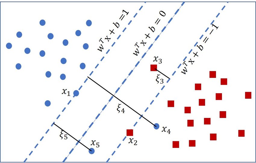
To account for the misclassifications, we introduce a slack variable $\xi_i \ge 0$ for each observation:
$$ \xi_i \approx \max(0, 1 - y_i (\mathbf{w}^\top \mathbf{x}_i + b)) $$
The right side of the $\approx$ is called the hinge loss. We use the approximate sign because the slack variable is not exactly the hinge loss, but some constant times the hinge loss.
If the observation is misclassified $y_i (\mathbf{w}^\top \mathbf{x}_i + b)$ will be negative, and the slack variable will be greater than 1. If the observation is correctly classified, but is within the margin, the slack variable will be between 0 and 1. The rest of the observations will have $\xi_i = 0$.
Geometrically, $\xi_i$ captures the distance from the correct side of the margin defined by the support vectors to the observation, which is an intuitive penalty for misclassification.
We obviously want this slack variable to be minimized.
With this slack variable, we now have a new constraint:
\[\begin{align*} \mathbf{w}^\top \mathbf{x}_i + b &\geq 1 - \xi_i & \text{if } y_i = +1 \\ \mathbf{w}^\top \mathbf{x}_i + b &\leq -1 + \xi_i & \text{if } y_i = -1 \end{align*}\]This soft-margin contraint can be compactly written as:
\[y_i (\mathbf{w}^\top \mathbf{x}_i + b) \geq 1 - \xi_i\]Notice that now our constraint is now loosened by its misclassified distance.
Since now we have two things to minimize, the original objective in addition to the sum of the slack variables, so we solve the following minimization problem:
$$ \min_{\mathbf{w}, b, \xi} \frac{1}{2} \lVert \mathbf{w} \rVert^2 + C \sum_{i=1}^{n} \xi_i \quad s.t.\quad y_i (\mathbf{w}^\top \mathbf{x}_i + b) \geq 1 - \xi_i, \quad \xi_i \geq 0 $$
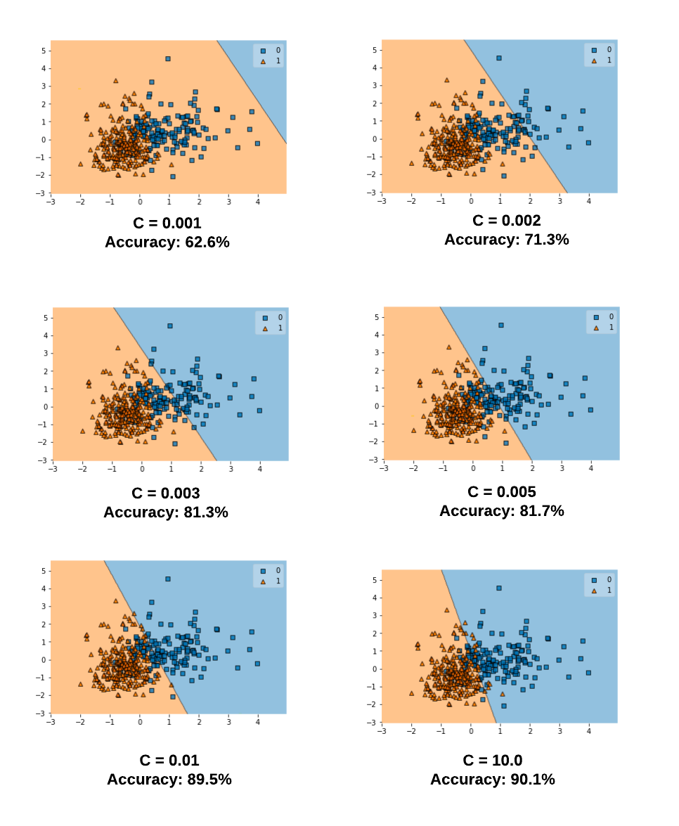
where $C$ is a hyperparameter that controls the trade-off between having a large, complex model (added $\xi_i$) and allowing more mistakes.
This $C$, much like a regularization variable, is chosen by cross-validation.
- With a huge $C$, we are essentially solving a hard-margin problem.
- Because in attempt to minimize the slack sum with a huge $C$, we will end up allowing slacks of near-zero values which is as rigid as a hard-margin.
- With a small $C$, we are giving more rooms for slack during the minimization.
SVC as an Inner Product
SVM optimization problem can be solved by Lagrange multiplier method.
Which leads to a inner product representation of the SVC.
Long story long
We have the objective function to minimize and a constraint function.
The objective function is bound to the constraint, meaning it’s gotta touch the constraint function at some point.
At this tangent point, the gradient of the objective function and the gradient of the constraint function are parallel (may be different directions and magnitudes, but on a same line).
Lagrange multiplier is a $\lambda$ multiplied to the constraint gradient to make it identical to the objective gradient.
The objective, constraint, and the Lagrange multiplier are combined to form a Lagrangian function, and we try to minimize this Lagrangian.
For the optimal solution, just like any minimization, we just solve for when the gradient of the Lagrangian is zero.
This Lagrangian is the called the primal form of the optimization problem, or primal problem. There is actually a dual form of the optimization problem.
This is a very rough idea of what’s going on.
The objective function and the multipliers kind of fight each other just like models with regularization fight between the objective and the penalty.
In the primal sense, we try to minimize the Lagrangian by minimizing over original variables. But we could achieve the same by maximizing over the multipliers.
Why the hell do we do this? Because turns out the dual form for SVM linear support vector classifier can be computed simply with inner products of the observations $\langle \mathbf{x}_i, \mathbf{x}_j \rangle$.
The classifier can also be expressed as:
\[f(\mathbf{x}) = \beta_0 + \sum_{i \in S} \hat{\alpha}_i \langle \mathbf{x}, \mathbf{x}_i \rangle\]where $S$ is the support set indices where ${\alpha}_i > 0$ (observations on and within the margin).
This is great computationally, but also essential for the kernel trick that we will see in the next section.
Kernel trick
Another way to solve non-linearly separable classifications is to use the kernel trick to transform the data.
Commonly used method to solve non-linearly separable classifications is to use the kernel trick in conjunction with the soft-margin SVC.
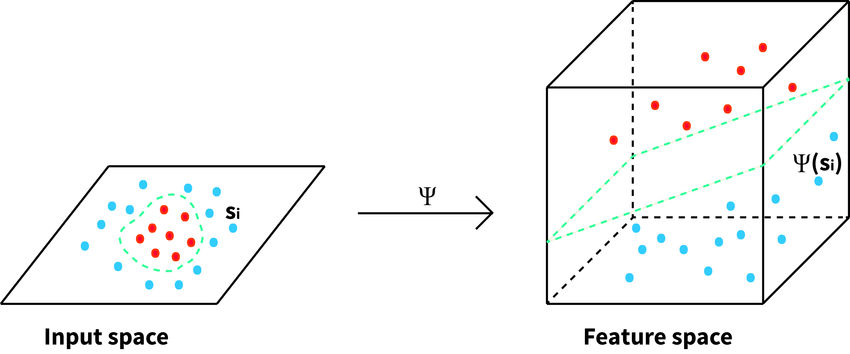
Let feature map $\Phi$ be a non-linear transformation that maps the data from a lower-dimensional input space to a higher-dimensional feature space.
$$ \Phi: \mathbb{R}^p \rightarrow \mathbb{R}^q \quad \text{where}\quad q > p $$
Cover's theorem
Cover’s theorem states that a linearly non-separable dataset in a lower-dimensional space may be linearly separable in a higher-dimensional space.
Kernel $K(\cdot)$ is a generalization of an inner product that satisfies the following:
$$ K(\mathbf{x}_i, \mathbf{x}_j) = \Phi(\mathbf{x}_i)^\top \Phi(\mathbf{x}_j) \quad \forall \mathbf{x}_i, \mathbf{x}_j \in \mathbb{R}^p $$
In other words, the kernel function is a function that given any two vectors in the input space, computes the dot product of them in the feature space.
Loose intuition
In the usual input space, the optimal solution given by the Lagrange multiplier method involves calculating the dot product of the observations $\mathbf{x}_i^\top \mathbf{x}_j$.
Since we now inflate the input space to a higher-dimensional feature space, we need to calculate the dot product of the observations in the feature space.
So in order to replace the inner product of inputs, we need to find a kernel that can compute the dot product of the observations in the feature space for all possible pairs of observations.
One key point is that as long as we can find a kernel with output that lives in the inner product space, we don’t have to have an explicitly defined feature map $\Phi$.
Radial basis function (RBF) kernel
Most commonly used kernel for SVC is the radial basis function (RBF) kernel.
The RBF kernel is defined as:
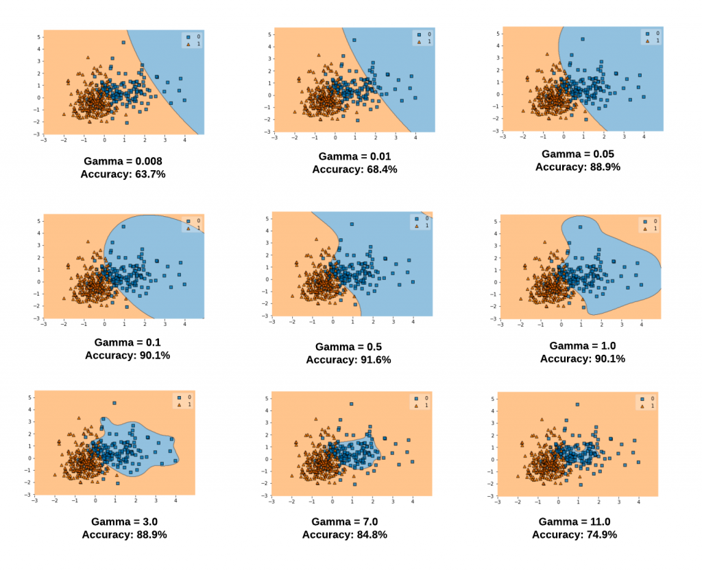
\[K(\mathbf{x}_i, \mathbf{x}_j) = \exp \left( -\frac{\lVert \mathbf{x}_i - \mathbf{x}_j \rVert^2}{2 \sigma^2} \right)\]$\sigma$ is a free variable that controls the flexibility of the decision boundary.
Oftentimes, we define
\[\gamma = \frac{1}{2 \sigma^2}\]Again, $\frac{1}{2}$ in the denominator is just for convenience. You may find $\gamma = \frac{1}{\sigma^2}$ in other sources.
so that the RBF kernel is defined as:
$$ K(\mathbf{x}_i, \mathbf{x}_j) = \exp \left( -\gamma \lVert \mathbf{x}_i - \mathbf{x}_j \rVert^2 \right) $$
where $\gamma > 0$.
Intuition
When two observations are close to each other, the sum of squared differences will be small, making the entire kernel value larger.
When two observations are far from each other, the sum of squared differences will be large, making the entire kernel value smaller.
SVC replaced with the RBF kernel is represented as:
\[f(\mathbf{x}) = \beta_0 + \sum_{i \in S} \hat{\alpha}_i K(\mathbf{x}, \mathbf{x}_i)\]If the new observation $\mathbf{x}$ is far from the support vectors, the kernel value will be small, and the contribution to the prediction will be small.
So the RBF kernel shrinks the contribution of the support vectors as observation moves away from them.
- Low $\gamma$: decision boundary is less flexible, more linear
- High $\gamma$: decision boundary is more flexible
Support Vector Regression
Support vector regression (SVR) is a regression model using the similar concept as the soft margin SVC.
What we do is try to fit a hyperplane that minimizes the residuals, while allowing some slack.
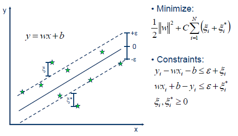
In soft margin SVC, we had the hinge loss to define the slack variable.
In SVR, we use the $\varepsilon$-insensitive loss to define the slack variable:
$$ \xi_i \approx max(0, \lvert y_i - \hat{y}_i \rvert - \varepsilon) $$
where $\hat{y}_i$ is the predicted value for $y_i$:
\[\hat{y}_i = \mathbf{w}^\top \mathbf{x}_i + b\]While the hinge loss penalizes any deviation from the correct side of the margin, the $\varepsilon$-insensitive loss only penalizes the deviation that is greater than the tube of width $2\varepsilon$ around the hyperplane.
We are insensitive to the residuals within $\varepsilon$ distance. Hence the name.