RNN
See Language Model & n-gram for basics of language modeling and shortcomings of non-neural language models.
Table of contents
Fixed-Window Neural Language Model
Recall that a langauge modeling task takes in a sequence of words and outputs the probability distribution of the next word.
With the same Markov assumption as in n-gram models, we can take a fixed-size window of words (embeddings) as input, put it through a hidden layer, and output the probability with a softmax.
Same stuff, but the only difference is that while it was important for n-gram models to actually see the precise n-gram in the corpus, neural models can generalize better on unseen n-grams.
No sparsity problem as in n-gram models.
It is also more compact than n-gram models because we do not have to store the counts of n-grams.
However, the fixed-size window is still a limitation.
Recurrent Neural Networks
Recurrent Neural Networks (RNNs) can handle sequences of arbitrary length.
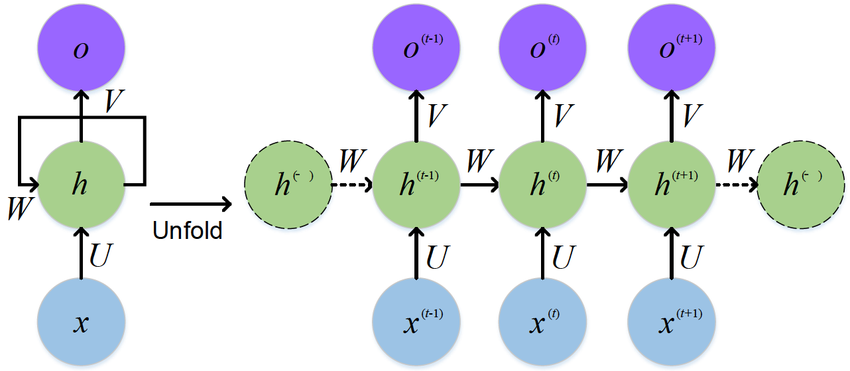
At each position, it takes the word embedding at timestep $t$ and the hidden state at timestep $t-1$ as input.
The same weight $W$ is reused at each step.
Word and Word Embedding
$\boldsymbol{x}^{(t)}$ is the one-hot encoding of the word at timestep $t$.
We will obtain the word embedding $\boldsymbol{e}^{(t)}$ by multiplying $\boldsymbol{x}^{(t)}$ with a word embedding matrix $\boldsymbol{E}$:
$$ \boldsymbol{e}^{(t)} = \boldsymbol{E} \boldsymbol{x}^{(t)} $$
Hidden State
$\boldsymbol{h}^{(0)}$ is the initial hidden state. It is usually initialized to zero.
And at each timestep $t$:
$$ \boldsymbol{h}^{(t)} = \tanh\left( \boldsymbol{W}_h \boldsymbol{h}^{(t-1)} + \boldsymbol{W}_e \boldsymbol{e}^{(t)} + \boldsymbol{b}_h \right) $$
Output
A vector of probabilities over the vocabulary, $\mathbb{R}^{|V|}$:
$$ \hat{\boldsymbol{y}}^{(t)} = \text{softmax}\left( \boldsymbol{W}_y \boldsymbol{h}^{(t)} + \boldsymbol{b}_y \right) $$
Advantages and Disadvantages
Advantages
- Handle sequences of arbitrary length.
- Model size doesn’t grow with input length.
Disadvantages
- Computation is slow.
- Performance degrades in the long term.
Cross-Entropy Loss
On each step $t$, we output the distribution of the next word $\hat{\boldsymbol{y}}^{(t)}$.
The loss function at step $t$ is the cross-entropy loss. The true distribution is $\boldsymbol{y}^{(t)}$ is the one-hot encoding of the next word $\boldsymbol{x}^{(t+1)}$:
$$ \begin{align*} J^{(t)}(\theta) &= - \sum_{w \in V} y_w^{(t)} \log \hat{y}_w^{(t)} \\[1em] &= - \log \hat{y}_{x^{(t+1)}}^{(t)} \tag{$\boldsymbol{y}^{(t)}$ is one-hot} \end{align*} $$
Total loss is the average of all step losses:
$$ J(\theta) = \frac{1}{T} \sum_{t=1}^T J^{(t)}(\theta) $$