Autocorrelation
Table of contents
What is autocorrelation?
Autocorrelation is a measure of how correlated a time series data is with the lagged version of itself.
While regular correlation measure the relationship between two different variables, autocorrelation measures the relationship between variables $X_t$ and $X_{t-k}$, where $k$ is the lag.
\[\rho(k) = \frac{\Cov[X_t, X_{t-k}]}{\sqrt{\Var[X_t] \Var[X_{t-k}]}}\]But assuming that the process is stationary (i.e. mean and variance are constant), the autocorrelation can be simplified to:
$$ \rho(k) = \frac{\Cov[X_t, X_{t-k}]}{\Var[X_t]} $$
ACF and PACF
Autocorrelation Function (ACF)
Autocorrelation Function (ACF) is autocorrelation as a function of lagged difference.
So obviously, at lag $0$, ACF is always $1$. This trivial result is disregarded.
ACF includes both direct correlation and indirect/conditional correlation between $X_t$ and $X_{t-k}$.
For example, in calculation of ACF for lag $2$, the direct correlation between $X_t$ and $X_{t-2}$, as well as the indirect correlation between $X_t$ and $X_{t-1}$ and between $X_{t-1}$ and $X_{t-2}$, all contribute to the ACF.
ACF is symmetric for positive and negative lags, so only positive lags are plotted.
Periodicity of ACF
ACF of a periodic process has the same periodicity as the original process.
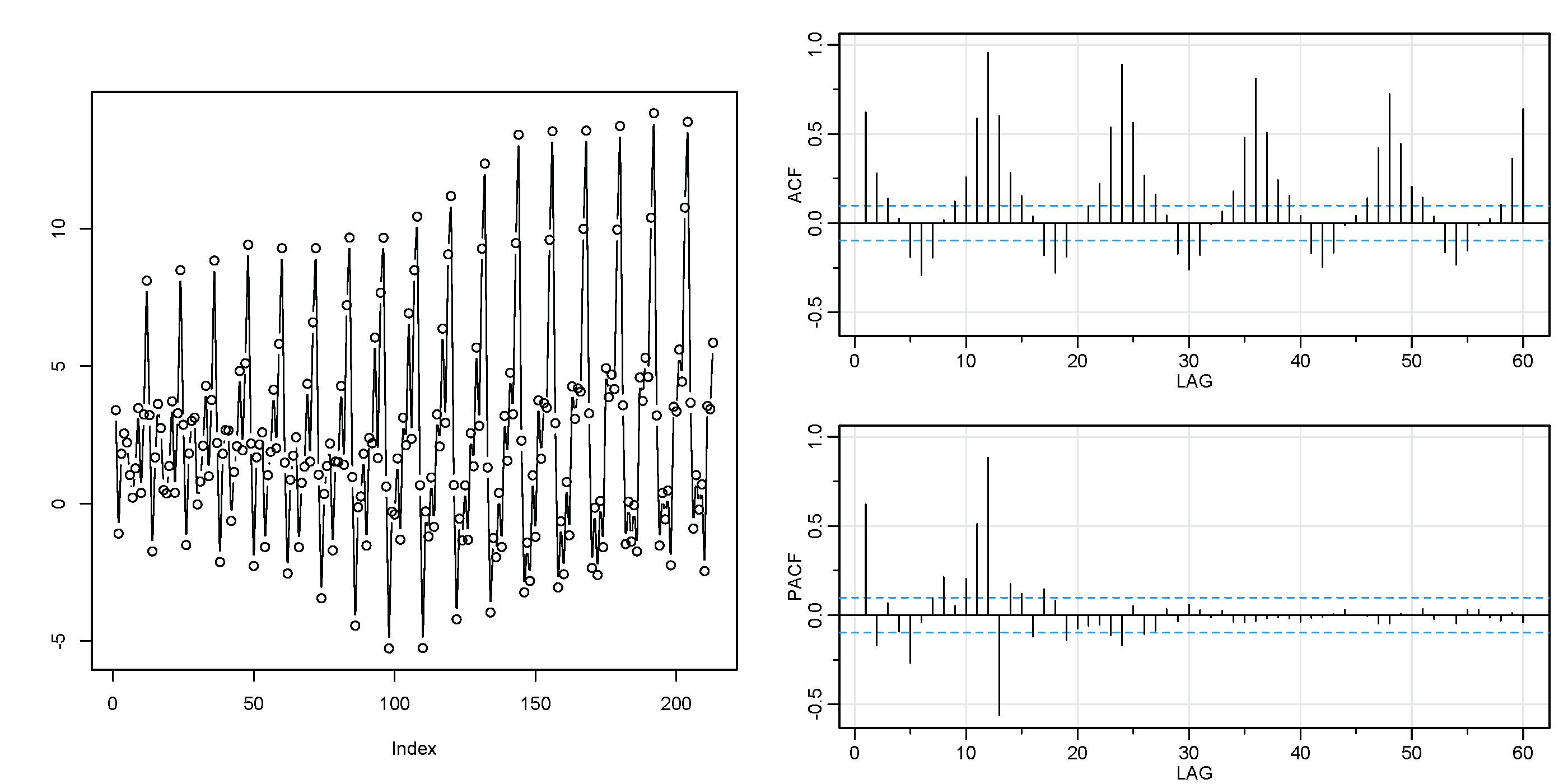
Therefore there can be repeating patterns in ACF (take a look at the correlogram above).
Additive property
For two periodic process $X_t$ and $Y_t$, $ACF(X_t + Y_t) = ACF(X_t) + ACF(Y_t)$.
Identifying stationarity with ACF
For stationary process, ACF quickly decays to $0$ as lag increases.
If it does not, the process is non-stationary. In that case you should try things like plotting the ACF of the differenced data (remove trend).
Statistical significance of sample ACF
Correlograms are often plotted with bands which indicate the critical values for statistical significance of AC.
Due to randomness in the data, we rarely get exactly zero for AC. Even for white noise data, we get non-zero values even though there is no autocorrelation between the data points.
Therefore, for some significance level, ACs that fall within the confidence interval are considered to be $0$ and thus not statistically significant.
Standard normal white noise
For standard normal white noise
\[X_t \sim \mathcal{N}(0, 1)\]theoretically AC is expected to be $0$.
So the 95 confidence interval for AC is
\[0 \pm {1.96} \times \frac{1}{\sqrt{n}}\]where $n$ is the sample size or the length of time series.
Although this calculation is based on the assumptions of standard normality (standard error of the mean is $\frac{1}{\sqrt{n}}$), seems like it is quite often used as a test of randomness on other time series data as well.
Without enough sample size, this test becomes too conservative.
General hypothesis test
In general, the statistical significance of AC under the null hypothesis that AC is zero (there is no correlation) and significance level $\alpha$ is estimated with:
$$ \pm z_{\alpha/2} \times SE(\hat{\rho}(k)) $$
where $\hat{\rho}(k)$ is the sample autocorrelation at lag $k$.
The standard error depends on the actual sample AC of the data and there are approximation methods to estimate it.
These are usually represented by shaded areas in ACF plots.
Partial Autocorrelation Function (PACF)
Partial Autocorrelation Function (PACF) is basically ACF with the indirect/conditional correlation removed.
Unlike ACF, PACF only considers the direct correlation between $X_t$ and $X_{t-k}$.
PACF controls other intermediate lags by including them as regressors.
For example, for lag $2$, PACF fits the following regression model:
\[y_t = \beta_0 + \beta_1 y_{t-1} + \beta_2 y_{t-2} + \epsilon_t\]Then outpus $\beta_2$ as the PACF for lag $2$, the direct effect of $y_{t-2}$ on $y_t$.
Because of this, PACF is used as a heuristic to determine the order of AR models. However, this heuristic can be used only if data is stationary. For data with a lot of random noise, PACF gets harder to interpret because it won’t diminish.
PACF is not periodic
Unlike ACF which carries the periodicity of the original process, PACF does not carry this redundancy.
Therefore sum of two periodic processes is not additive unlike ACF.
Identifying non-stationarity with PACF
For a trending non-stationary process, the value at lag $1$ is often positive and large and the values at other lags are not statistically significant.
This can be interpreted as that the only thing affecting each data point is the previous data point.
The previous point contains all the information that is needed to predict the next point, which typically indicates a trend.
Statistical significance of sample PACF
It is calculated in the same way as ACF.