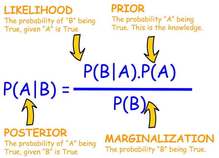
Bayes’ Theorem
Table of contents
Marginal Probability
A marginal probability is the probability of an event occurring, irrespective of other events.
So simply put, it is the probability of an event without any conditions.
This term is used in contrast to a conditional probability, which is the probability of an event that depends on other events.
The Law of Total Probability
The law of total probability is a theorem that relates marginal probabilities to conditional probabilities.
If $A_i$ is a partition of a sample space $\Omega$, then for any event $B$ in $\Omega$,
$$ P(B) = \sum_{i} P(B|A_i)P(A_i) $$
Marginalization
Marginalization is the process of summing over all possible values of a variable to find the marginal distribution of another variable.
$$ P(B) = \sum_{i} P(B, A_i) $$
So it’s basically the same idea as the law of total probability, but without the conditionals.
Interpreting Bayes’ Theorem
Let $A_i$ be a partition of a sample space $\Omega$.
Then for any event $B$ in $\Omega$, Bayes’ theorem states that:
$$ P(A_i|B) = \frac{P(B|A_i)P(A_i)}{P(B)} = \frac{P(B|A_i)P(A_i)}{\sum_{j} P(B|A_j)P(A_j)} $$
In Bayesian statistics, probability is interpreted as a measure of belief.
So this rule tells us how our beliefs are updated given new observations.
Prior
A prior is a probability distribution that represents our beliefs prior to observing any new data.
So in our case $P(A_i)$ is the prior.
In Bayesian inference, the prior is often initialized to a uniform distribution as a non-informative prior (i.e. no prior knowledge, less bias).
Posterior
A posterior is a probability distribution that represents our beliefs after observing new data.
In our case $P(A_i | B)$ is the posterior.
The new observation is represented by $B$, and $P(A_i | B)$ is our updated belief about $A_i$.
Marginal
In real life, we often have no direct way to solve for $P(B)$.
In this case, the entire posterior is approximated using methods such as MCMC (Markov Chain Monte Carlo).
