Method of Lagrange Multipliers
Popular method to solve constrained optimization problems.
Lagrange Multipliers
Optimization problem with constraints is often defined as follows:
- Objective function to be maximized or minimized
- Constraint(s) that must be satisfied
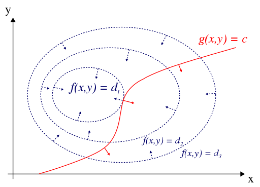
In the case of the figure above, the objective function is $f(x,y)$ and the constraint is $g(x,y) = c$.
Very rough idea is as follows:
Out of the many level curves $f(x,y) = d$ can take, we want to pick the one with maximum or minimum $d$.
Since we have a constraint, we can only expand or shrink the curve until it touches the constraint $g(x,y) = c$.
There should be a point where both curves become tangent to each other.
At this tangent, $f(x,y)$ is at a local extreme while satisfying the constraint.
The gradient vector $\nabla f(x,y)$ is orthogal to its tangent vector, and so is the gradient vector $\nabla g(x,y)$ to its tangent vector.
Although they may be in opposite directions and/or different magnitudes, both gradient vectors are aligned.
In the figure above, they are the blue dotted line vector and the red line vector at the tangent point facing opposite directions.
If we scale the gradient vector $\nabla g(x,y)$ by a constant $\lambda$, we can make it equal to the gradient vector $\nabla f(x,y)$.
$$ \nabla f(x,y) = \lambda \nabla g(x,y) \quad \Rightarrow\quad \nabla f(x,y) - \lambda \nabla g(x,y) = 0 $$
This constant $\lambda$ is called the Lagrange multiplier, and $(x,y)$ that satisfies the above equation is the optimal solution.
Multiple constraints
When there are multiple constraints, i.e. $g_i(x,y) = c_i$, we can extend the above equation as follows:
$$ \nabla f(x,y) = \sum_{i=1}^{m} \lambda_i \nabla g_i(x,y) \quad \Rightarrow\quad \nabla f(x,y) - \sum_{i=1}^{m} \lambda_i \nabla g_i(x,y) = 0 $$
where $m$ is the number of constraints.
$\lambda_i$ are the set of Lagrange multipliers.
Lagrangian
You may be wondering where the actual constraint constant of each $g_i(x,y) = c_i$ went.
Because that information is not captured in the equation above.
In fact, the above system of equations does not provide enough information to solve for the optimal solution, because now we have added $m$ more unknowns $\lambda_i$, while the gradient vectors $\nabla f(x,y)$ and $\nabla g_i(x,y)$ only provide enough for $x$ and $y$.
We want to package the information of the constraints into the system of equations.
The Lagrangian is the function that accomplishes this.
$$ \mathcal{L}(x,y,\lambda) = f(x,y) - \sum_{i=1}^{m} \lambda_i (g_i(x,y) - c_i) $$
To solve for the optimal solution, now you just need to solve:
$$ \nabla \mathcal{L}(x,y,\lambda) = 0 $$
\[\nabla \mathcal{L}(x,y,\lambda) = \begin{bmatrix} \frac{\partial \mathcal{L}}{\partial x} \\ \frac{\partial \mathcal{L}}{\partial y} \\ \frac{\partial \mathcal{L}}{\partial \lambda_1} \\ \vdots \\ \frac{\partial \mathcal{L}}{\partial \lambda_m} \end{bmatrix} = \vec{0}\]Lagrangian dual function
To be added
The above Lagrangian is the primal form of the optimization problem.
There is actually a dual form of the optimization problem.
Say our goal was to minimize the Lagrangian above:
The primal approach above is to minimize the first part by minimizing over the primal variables $x$ and $y$ while adhering to the second part.
Or we could try to maximize the second part by maximizing over the dual variable $\lambda$ while adhering to some constraints which are derived from the primal variables.
Why would we want to do this?
Turns out, sometimes the dual form is easier to solve than the primal form.
