MST Algorithms
Table of contents
Minimum Spanning Trees
Review the concept of MST.
Assume Unique MST
When edges do not have distinct weights, the MST is not unique. This complicates proof of correctness for MST algorithms.
However, without loss of generality, we can assume that all edge weights are unique.
We will see why when we discuss the light-edges.
Zero or Negative Weights are Allowed
Unlike some shortest path algorithms, MST algorithms can handle zero or negative edge weights.
Cut
A cut of a connected, undirected graph $G = (V, E)$ is a partition of $V$ into two sets:
$$ (S, V \setminus S) $$
It is defined in terms of $S$ which is a non-empty proper subset of $V$:
\[S \neq \emptyset \land S \subsetneq V\]
Crossing Edge
An edge $(u, v)$ crosses the cut if:
$$ u \in S \land v \in V \setminus S $$

Respecting Edge Sets
For some set of edges $A$, we say that a cut respects $A$ if no edge in $A$ crosses the cut.
For example, in the figure above, our cut respects $\{(a,b), (b,e)\}$.
Light Edge
The minimum-weight edge that crosses a cut is called a light edge.

Why we can assume unique edge weights
We mentioned earlier that we can w.l.g. assume that edge weights are distinct, to ensure that the MST is unique and still prove correctness.
This works because MST algorithms are basically about finding the lightest edge on each round of the algorithm.
If two edges have the same weight, we can just theoretically enforce a certain tie-breaking rule so that our algorithm behaves as if the weights were distinct.
In the case above, suppose all our crossing edges had weight of $2$. Then I would just say, “okay on this round, select the rightmost edge”, which would select our desired edge $(e,f)$.
Light-Edge Property / Safe Edge
The light-edge property states that:
$(u,v)$ is a light edge for a cut $\Rightarrow$ $(u,v)$ belongs to the MST.
Another way to phrase this is through the concept of a safe edge.
Let $A$ be a set of edges that is a subset of some MST $T$.
So we have a valid subset of the MST so far.
Let there be a cut that respects $A$, and let $(u,v)$ be a light edge for that cut.
Then $(u,v)$ is a safe edge for $A$.
Safe as in, adding it to $A$ will not violate the MST requirement, and thus belongs to the MST.
Proof
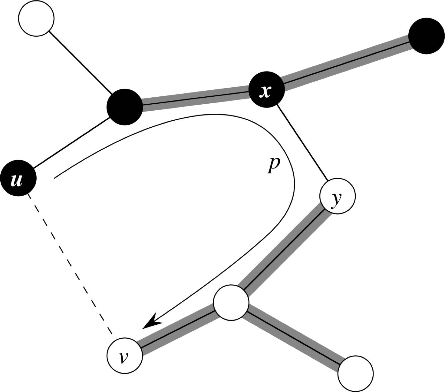
Suppose $(u,v)$ does not belong to the MST $T$, which includes edge set $A$.
Adding $(u,v)$ must create a cycle, so there is already a path $p(u,v)$ in $T$.
$(u,v)$ is a crossing edge for the cut, so there must be some edge $(x,y)$ in $p(u,v)$ that crosses the cut.
Because the cut respects $A$, $(x,y) \notin A$ so far.
Removing $(x,y)$ from $T$ partitions $T$ into two trees, and adding $(u,v)$ connects them back. So we have a new spanning tree $T’$:
\[T' = T \setminus \{(x,y)\} \cup \{(u,v)\}\]However, $(u,v)$ is a light edge, so its weight is less than or equal to $(x,y)$, hence:
\[w(T') \leq w(T)\]Since $T$ is an MST:
\[w(T') \leq w(T) \land w(T) \leq w(T') \Leftrightarrow w(T') = w(T)\]Hence, $T’$ must also be an MST.
Since $(x, y) \notin A$, we can form an MST with $A \cup {(u,v)}$.
Two Classic MST Algorithms
- They are both greedy algorithms.
- They both find the optimal (true MST) solution.
- They both add one safe edge at a time.
- They are asymtptically equivalent in terms of time complexity.
- But for dense graphs, Kruskal’s is slightly slower than Prim’s.
Prim’s Algorithm
- Grows a single tree by continuously connecting a new vertex via a light edge.
- Involves a priority queue to keep track of light edges.
Pseudocode
def prim(V, E):
  visited = set()  # Vertices already in MST
  prev = { v: None for v in V }  # How are they going to be reached?
  pq = PriorityQueue(
    (None, v) for v in V  # Initialize with infinite cost
  )

  u = V[0]  # Start from any vertex
  pq.update((0, u))  # Cost, vertex

  while length(visited) < len(V):  # While not all vertices are visited
    _, u = pq.pop()  # Get the lightest edge
    visited.add(u)

    for v in E[u]:  # For each neighbor of u
      if v in visited:  # Skip if already visited
        continue
      # Update the cost in pq if there is a lighter edge
      if weight(u, v) < pq.get_cost(v):
        pq.update(weight(u, v), v)
        prev[v] = u  # Update how to reach v

  # Reconstruct the MST edges
  mst_edges = []
  while len(mst_edges) < len(V) - 1:
    mst_edges.append((prev[u], u))
    u = prev[u]

  return mst_edges
Given that graph is represented as an adjacency list and the priority queue is implemented as a binary heap, time complexity of Prim’s algorithm is:
- Initialization of priority queue with default values: $O(|V|)$.
- Pop from priority queue happens once per vertex: $O(|V| \log |V|)$.
- Update to priority queue happens at most twice per edge: $O(|E| \log |V|)$.
Assuming we have more edges than vertices, Prim’s algorithm has a time complexity of $O(|E| \log |V|)$.
Kruksal’s Algorithm
- Grows a forest of trees by continously adding a safe edge that connects two trees.
- These forests eventually merge into a single tree.
- Sorts edges by weight and adds them in increasing order.
- Uses priority queue to keep track of light edges.
- Uses disjoint-sets/union-find to keep track of connected components.
Psuedocode
def kruskal(V, E):
  uf = UnionFind(V)  # Initialize disjoint sets for each vertex
  pq = PriorityQueue(  # Initialize priority queue with all edges
    (weight(u, v), (u, v)) for u, v in E
  )
  mst_edges = []

  while pq:
    w, (u, v) = pq.pop()  # Get the lightest edge
    if uf.find(u) != uf.find(v):  # If they are not in the same set
      mst_edges.append((u, v))  # Add the edge to the MST
      uf.union(u, v)  # Merge the sets

  return mst_edges
Assuming that the priority queue is implemented as a binary heap, the complexity of Kruskal’s algorithm depends on the implementation of union-find.
Assuming that the amortized time complexity of union-find is $O(\log |V|)$:
- Initialization of disjoint sets: $O(|V|)$ (assuming
make_setis $O(1)$). - Pop from priority queue happens once per edge for sorting: $O(|E| \log |E|)$.
- $O(|V|)$ finds and $O(|E|)$ unions: $O((|V| + |E|) \log |V|)$.
Since we have more edges than vertices, $O(|E| \log |E|)$ dominates the time complexity.
However,
\[|E| \le |V|^2 \Rightarrow \log |E| = O(\log |V|)\]So the time complexity of Kruskal’s algorithm is $O(|E| \log |V|)$.