Single Source Shortest Path
One type of the shortest path problem.
Dijkstra’s and Bellman-Ford algorithms are two of the most well-known algorithms.
Table of contents
Problem Definition
We are given a source vertex $s \in V$.
The single-source shortest-paths problem (SSSP):
Find the shortest path from $s$ to every other vertex $v \in V$.
The result is a shortest path tree rooted at $s$.
The following variants can be reduced to the single-source problem:
- Single-Destination: Find the shortest path to a given vertex.
- Reverse the direction of all edges
- Single-Pair: Find the shortest path between two given vertices.
- Trivially solved
However, all-pairs is (sort of) a different setting. It is solvable by running the single-source algorithm once for each vertex, but the time complexity is improved by a different algorithm. We will discuss it later.
General Algorithm Structure
- Each vertex $v$ stores two attributes:
- Distance $v.d$: the tentative shortest path weight estimate from $s$ to $v$
- Predecessor $v.\pi$: the vertex preceding $v$ in the tentative shortest path
We want to be able to reconstruct the path, that’s why we store the predecessor.
SSSP algorithms initialize distance estimate and tentative predecessor for each vertex, then iteratively relax edges to improve the estimates.
Initialization
def init_single_source(G, s):
  for v in G.V:
    v.d = float('inf')
    v.p = None
  s.d = 0
$O(|V|)$ time complexity.
Relaxation
Relaxing an edge $(u,v)$ tests whether our shortest path estimate $v.d$ can be improved by $u.d + w(u,v)$ (going through $u$).
If going through $u$ is better, update $v$:
def relax(u, v):
  if v.d > u.d + w(u, v):
    v.d = u.d + w(u, v)
    v.p = u
On the term "Relaxation"
I found the term “relaxation” a bit confusing, so I decided to think of it as a bezier curve.
You had a pretty rigid bezier curve to $v$. But you add control point $u$ which makes the curve smoother and relaxes the curve to $v$.
Path-Relaxation Property
Let path $p = (v_0, v_1, \ldots, v_k)$ where $w(p) = \delta(v_0, v_k)$
In other words, $p$ is the shortest path from $v_0$ to $v_k$.
If we relax the edges of $p$ in order $(v_0, v_1), (v_1, v_2), \ldots, (v_{k-1}, v_k)$, then $v_k.d = \delta(v_0, v_k)$.
The important thing is that these relaxations do not need to be done in a strictly sequential order. Relaxations on any other edges can be interleaved.
Proof by Induction
- Base case: $k = 0$: Trivially, $v_0.d = 0 = \delta(v_0, v_0)$.
- Inductive hypothesis: $v_{k-1}.d = \delta(v_0, v_{k-1})$.
- Inductive step:
We now relax $(v_{k-1}, v_k)$.
This means that now $v_k.d = v_{k-1}.d + w(v_{k-1}, v_k)$.
By the inductive hypothesis,
\[v_k.d = \delta(v_0, v_{k-1}) + w(v_{k-1}, v_k) = \delta(v_0, v_k)\]This property is crucial for the correctness of the algorithms below.
The algorithms somehow manage to relax the edges in the topological order defined by the shortest path, which is why they work.
Shortest Path is Always Well-Defined in DAG
Directed Acyclic Graphs (DAGs) is just a tree with directed edges. So we can always find a topological order of the vertices.
By logic, the shortest path has to be in this topological order, otherwise, it would not be the shortest path.
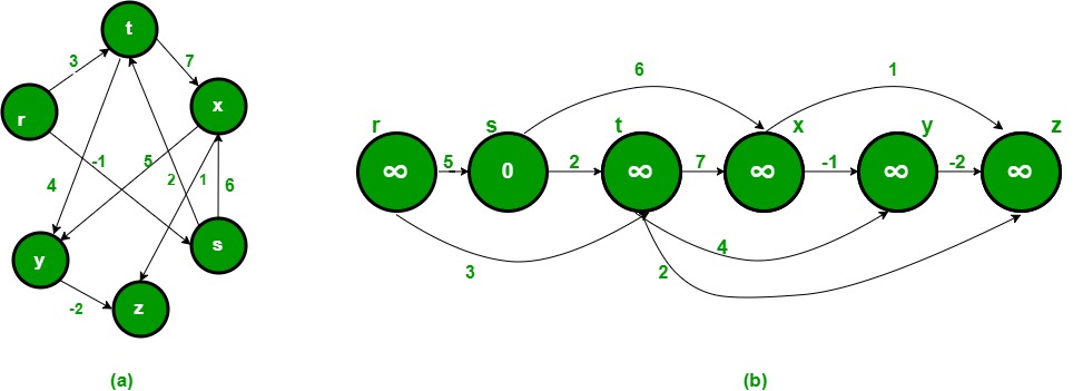
If we do a topological sort of the vertices and edges, and relax the edges in this order, by the path-relaxation property, we can always find the shortest path in a DAG.
How to Find the Topological Order?
The question now is how do we find the topological order?
One way to do this is to use depth-first traversal (DFT).
def topo_sort(G):
  order = []
  for v in G.V:
    v.visited = False
  for v in G.V:
    if v.visited == False:
      df_visit(G, v, order)

  return reversed(order)

def df_visit(G, u, order):
  u.visited = True
  for v in G.adj[u]:
    if v.visited == False:
      df_visit(G, v)
  order.append(u)
Dijkstra’s Algorithm
- Dijkstra’s algorithm is a greedy algorithm.
- Dijkstra’s algorithm works for non-negative edge weights.
- Dijkstra’s algorithm is optimal.
- Dijkstra’s algorithm is not optimal for negative edge weights.
- Dijkstra’s algorithm relaxes each edge once.
- Dijkstra’s algorithm uses a minimum priority queue.
- Generalization of BFS to weighted graphs.
Pseudocode
def dijkstra(G, s):
  init_single_source(G, s)  # O(V)

  S = set()
  Q = PriorityQueue()
  for v in G.V:  # O(V), since no heapify
    Q.put(v)

  while not Q.empty():
    u = Q.get()
    for v in G.adj[u]:
      # Relaxation with PQ update
      if v.d > u.d + w(u, v):
        v.d = u.d + w(u, v)
        v.p = u
        Q.update(v)  # Decrease-key operation
    S.add(u)
This algorithm has a time complexity of $O((V+E) \log V)$:
Q.get()called $O(V)$ times: $O(V \log V)$Q.update()called $O(E)$ times: $O(E \log V)$
If given graph is dense, $O(E \log V)$.
See C++ implementation here.
Bellman-Ford Algorithm
While Dijkstra’s algorithm relaxes one edge with the smallest shortest path estimate at a time, Bellman-Ford relaxes all edges in each iteration.
- Bellman-Ford is slower than Dijkstra’s algorithm.
Bellman-Ford is optimal even for negative edge weights.
You can mandate a certain edge to be selected by giving it a large negative weight $-\infty$.
- Bellman-Ford can be parallelized.
- Per each vertex
- Bellman-Ford can detect negative-weight cycles.
Psuedocode
def bellman_ford(G, s):
  init_single_source(G, s)  # O(V)

  for _ in range(G.V - 1):  # We will reason why this is enough
    for u, v in G.E:
      relax(u, v)

  # The above steps should have saturated the shortest paths
  # If not, there is a negative-weight cycle
  for u, v in G.E:
    if v.d > u.d + w(u, v):  # Further relaxation possible
      return False  # Negative-weight cycle

  return True
- We relax $|E|$ edges $|V| - 1$ times, $O(|V| \cdot |E|)$.
Why $|V| - 1$ iterations?
How do we know that after $|V| - 1$ iterations, Bellman-Ford algorithm has found the shortest path?
Exploiting the Path-Relaxation Property
Bellman-Ford exploits the path-relaxation property above by relaxing all edges in each iteration.
Shortest path is acyclic and thus a tree of all vertices in the graph, which means it will contain $|V| - 1$ edges.
Every edge is relaxed at each iteration, and there are $|V| - 1$ iterations.
So Bellman-Ford covers every permutation of the relaxation orders. So it is guaranteed to find the shortest path.
See C++ implementation here.