Distributional Representation of Words
Table of contents
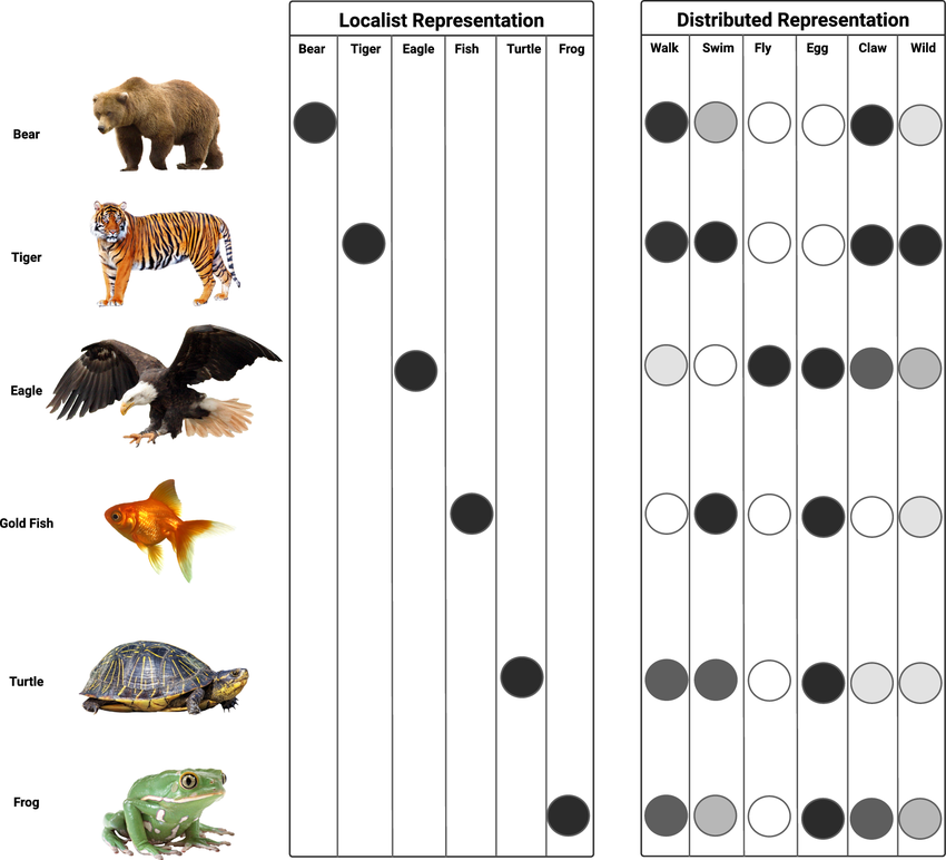
Localist Representation
In a localist representation, we treat each word as a discrete symbol. One-Hot Encoding vector is an example of localist representation.
The disadvantage of localist representation is:
- Vector size grows with the vocabulary size
- No notion of similarity between words
A solution to this is to use distributed representation, where each word is represented by a pattern across multiple other words.
In other words, the meaning of a word is distributed across multiple dimensions.
Distributional Semantics
Unlike lexical semantics, which focuses on the inherent meaning, usage, and relation of words, distributional semantics analyzes the meaning of words from their distribution in a corpus (from the context in which they appear).
Lexical representation of semantics is usually done via manual construction, whereas distributional representation is done automatically from corpora.
Distributional Hypothesis
Distributional representation is based on the distributional hypothesis, which suggests that
Words with similar meanings tend to occur in similar contexts.
Window Size and Context
We are usually given a corpus, which is often a raw dump of text. It can also come in multiple preprocessed forms (trees, etc.).
The context of a word in a corpus is the set of words around it.
The window size determines how many words to the left and right of the target word are considered part of the context.
Count-Based Methods
Co-Occurrence Matrix
Given a corpus and a window size, each word in the vocabulary is represented by a vector that counts the number of times it co-occurs with other words.
In other words, you count how many times other words appear in the context of the word being represented.
For example, given i believe i can fly and a window size of 1, the co-occurence vector for the word i would be:
| Word | i | believe | can | fly |
|---|---|---|---|---|
| i | 0 | 2 | 1 | 0 |
Hence [0, 2, 1, 0].
The collection of these vectors forms a co-occurrence matrix $C$.
Pointwise Mutual Information (PMI)
There is a problem with the co-occurrence matrix:
Some words are just naturally more frequent than others (e.g., “the”)
We would want the word dog to have a higher relation with bark, but because of how frequent the dog is, we might end up with a higher relationship between the and dog.
We introduce Pointwise Mutual Information (PMI) to solve this problem.
Let $p_{xy}$ be the probability of words $x$ and $y$ co-occurring in a context. Let $p_x$ and $p_y$ be the probabilities of $x$ and $y$ occurring independently. Then:
$$ PMI(x, y) = \log \frac{p_{xy}}{p_x p_y} = \log \frac{C(x, y) \cdot N}{C(x) \cdot C(y)} $$
What?
\[\log \frac{p_{xy}}{p_x p_y} = \log \frac{\frac{C(x, y)}{N}}{\frac{C(x)}{N} \cdot \frac{C(y)}{N}} = \log \frac{C(x, y) \cdot N}{C(x) \cdot C(y)}\]Naturally frequent words are penalized in PMI, giving us a better representation.
Positive PMI (PPMI)
There is yet another problem with PMI: when $C(x, y) = 0$, $PMI(x, y) = \log 0 = -\infty$.
So, we use Positive PMI (PPMI):
$$ PPMI(x, y) = \max(0, PMI(x, y)) $$
Basically a rectified version of PMI.
TF-IDF
Downside of Count-Based Methods
- Large Matrix Size: grows with the vocabulary size
- Sparsity: most entries are zero
To solve this issue we often use PCA/SVD to reduce the dimensionality.
Another solution is to use neural networks to learn the embeddings, which we will see in the next section.
Dimensionality Reduction
Refer to the link below for details.
Principal Component Analysis (PCA)
Long story short:
Let $X$ be the PPMI matrix obtained from the corpus. Each row of $X$ is a word vector.
The issue is that $X$ is very large and sparse. We do SVD on $X$ to get $X = USV^T$.
We select a few principal components based on the singular values sorted in descending order (also known as proportion of variance explained), let’s say $p$.
We then take the first $p$ columns of $U$ as the word vectors, which results in a lower-dimensional representation of the words.