Word2Vec
Predictive models for learning word embeddings.
Our objective is to put relevant words close to each other in the vector space.
Table of contents
Problem with Distributional Representation
Distributional representation, or representation obtained from statistical, count-based methods like TF-IDF and PPMI are also based on the distributional hypothesis, just like Word2Vec.
However, statistical methods have some limitations:
- Large matrix sizes due to large vocabularies
We could use techniques like SVD to reduce the dimensionality. But an SVD on a $n \times n$ matrix has a time complexity of $O(n^3)$, which is unrealistic for large vocabularies.
Also, SVD is a full-batch algorithm, while Word2Vec can be trained on mini-batches, allowing it to handle large datasets.
Word2Vec produces a distributed representation of words.
Distributional vs Distributed Representation
Refer to this link.
In distributed representation, each word is represented by some $d$-dimensional dense vector.
Bag of Words Model
Word2Vec is a bag of words model.
This type of model ignores the position of words in a sentence. Whether a word appears at the beginning or the end of a sentence, the resulting word embedding will be the same.
Two Different Approaches
Word2Vec is a group of models used to produce word embeddings. It comes in two flavors:
- Continuous Bag of Words (CBOW): predict the target word given the context words
- Skip-Gram: predict the context words given the target word
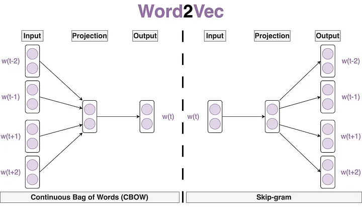
They are both shallow neural networks with a single hidden layer.
Skip-Gram
block-beta
  columns 10
  block:group1
  i1["i"] b["believe"] i2["?"] c["can"] f["?"]
  end
  style group1 fill:#fee,stroke:#333,stroke-width:2px
  style i2 fill:#fff,stroke:#333,stroke-width:1px,stroke-dasharray: 5, 5
  style f fill:#fff,stroke:#333,stroke-width:1px,stroke-dasharray: 5, 5
  style c fill:#f8b
Skip-Gram model creates word embeddings by predicting the context words based on the target word.
It learns by guessing the surrounding words.
- Slower to train than CBOW
- Works well with infrequent words
- Works well with smaller datasets
Let $t$ be the position of the target word. Let $m$ be the window size.
Then $w_t$ is the target word, and context words are $w_{t-m}, \ldots, w_{t-1}, w_{t+1}, \ldots, w_{t+m}$.
We want to maximize the likelihood of the context words given the target words:
\[L(\theta) = \prod_{t=1}^{T} \prod_{\substack{-m \leq j \leq m \\ j \neq 0}} P(w_{t+j} \mid w_t; \theta)\]Suppose we’ve preprocessed the corpus to obtain $D$, a set of word-context pairs.
Then the likelihoood can be rewritten as:
\[L(\theta) = \prod_{(w,c) \in D} P(c \mid w; \theta)\]The loss function (objective) is the negative log likelihood.
Probability of Context Given Target Word
We still need a way to model $P(c \mid w; \theta)$.
We will introduce two embedding vectors for each word $w$:
- $v_w$ when $w$ is the target word
- $u_w$ when $w$ is a context word
Implication
What this implies is that each word has different representations depending on whether it is used as a target (center) word or a context word.
Otherwise, the probability of a word being a context word of itself would end up being fairly high, due to the fact we’re using a dot product.
But in reality, $P(\text{dog} \mid \text{dog})$, the probability of seeing dog dog in a sentence should be very low.
The probability of a context word $c$ given a target word $w$ is modeled as a softmax:
$$ P(c \mid w; \theta) = \frac{\exp(u_c^T v_w)}{\sum_{x \in V} \exp(u_x^T v_w)} $$
where $V$ is the entire vocabulary.
We are measuring the similarity between a context and a target word with a dot product, and normalizing it over the entire vocabulary.
Gradient Descent
Our loss function is the negative log likelihood:
\[J(\theta) = - \sum_{(w,c) \in D} \log P(c \mid w; \theta)\]For a single pair $(w,c)$, the partial derivative of the loss function with respect to $v_w$ is:
\[\begin{align*} \frac{\partial J(\theta)}{\partial v_w} &= -\frac{\partial}{\partial v_w} \log P(c \mid w; \theta) \\ &= - \frac{\partial}{\partial v_w} \log \frac{\exp(u_c^T v_w)}{\sum_{x \in V} \exp(u_x^T v_w)} \\ &= - u_c + \sum_{x \in V} P(x \mid w; \theta) u_x \end{align*}\]What?
\[\begin{align*} \frac{\partial}{\partial v_w} \log \frac{\exp(u_c^T v_w)}{\sum_{x \in V} \exp(u_x^T v_w)} &= \frac{\partial}{\partial v_w} \left( u_c^T v_w - \log \sum_{x \in V} \exp(u_x^T v_w) \right) \\ &= u_c - \frac{1}{\sum_{x \in V} \exp(u_x^T v_w)} \cdot \sum_{x' \in V} \exp(u_{x'}^T v_w) u_{x'} \\ &= u_c - \sum_{x \in V} P(x \mid w; \theta) u_x \end{align*}\]As Cross-Entropy Loss
Let $\hat{y}$ be the model prediction for target word. Then $\hat{y}_x$ is the entry corresponding to word $x$.
Single pair loss function is:
\[J(\theta) = - \log P(c \mid w; \theta) = - \log \hat{y}_c\]Cross-entropy loss function is:
\[- \sum_{x \in V} y_x \log \hat{y}_x\]where $y$ is the one-hot encoded vector for the context word $c$.
Every $y_x$ is 0 except for $y_c$ which is 1:
\[- \sum_{x \in V} y_x \log \hat{y}_x = - \log \hat{y}_c\]Therefore, the softmax loss function is the same as the cross-entropy loss function between the true label and the model prediction.
Let $\hat{y}_v$ be the model prediction entry for word $v$ given word $w$:
\[- u_c + \sum_{x \in V} \hat{y}_x u_x\]Let $y$ be the one-hot encoded vector for the context word $c$ (the true label). Since $y_x = 1$ only when $x = c$, we can rewrite above as:
\[\begin{align*} - \sum_{x \in V} y_x u_x + \sum_{x \in V} \hat{y}_x u_x &= \sum_{x \in V} (\hat{y}_x - y_x) u_x \end{align*}\]Since it is a linear combination of the columns of the matrix $U$, we can write the gradient as:
\[\frac{\partial J(\theta)}{\partial v_w} = U (\hat{y} - y)\]The implication of this gradient is that upon gradient descent, we update the target word vector $v_w$ by the difference between the predicted context word vector $\hat{y}$ and the true context word vector $y$.
Minimizing this difference has the effect of bringing $v_w$ closer to the context word vector $u_c$.
We will skip the derivation of the gradient with respect to $u_c$. But the end result is similar: gradient descent will update the context word vector $u_c$ closer to the target word vector $v_w$.
CBOW
block-beta
  columns 10
  block:group1
  i1["i"] b["believe"] i2["?"] c["can"] f["fly"]
  end
  style group1 fill:#fee,stroke:#333,stroke-width:2px
  style i2 fill:#fff,stroke:#333,stroke-width:1px,stroke-dasharray: 5, 5
  style b fill:#f8b
  style c fill:#f8b
Continuous Bag of Words (CBOW) model creates word embeddings by predicting the target word based on the context words.
Essentially, the model learns by punching a hole and guessing the missing word.
- It is faster to train than Skip-Gram
- It works well with frequent words
Let $t$ be the position of the target word. Let $m$ be the window size.
Then $w_t$ is the target word, and context words are $w_{t-m}, \ldots, w_{t-1}, w_{t+1}, \ldots, w_{t+m}$.
We want to maximize the likelihood of the target words given the context words:
\[L(\theta) = \prod_{t=1}^{T} P(w_t \mid w_{t-m}, \ldots, w_{t-1}, w_{t+1}, \ldots, w_{t+m}; \theta)\]The loss function (objective) is the negative log likelihood.
Probability of Target Given Context Words
Similar to Skip-Gram, we introduce two vectors for each word $w$:
- $v_w$ when $w$ is the target word
- $u_w$ when $w$ is a context word
to model the probability.
However, unlike Skip-Gram, we will now calculate the average of the context word vectors:
\[\bar{u}_{context} = \frac{1}{2m} \sum_{-m \leq j \leq m, j \neq 0} u_{w_{t+j}}\]Remember $m$ is the window size.
The probability of a target word $w$ given the context words is
$$ P(w \mid \text{context}; \theta) = \frac{\exp(v_w^T \bar{u}_{context})}{\sum_{v \in V} \exp(v^T \bar{u}_{context})} $$
Issue with Word2Vec
Word2Vec requires a softmax layer with an input size equal to the vocabulary size.
If our vocabulary is huge (which is often the case), calculating the softmax becomes too expensive.
Remember, softmax requires a normalization over the entire vocabulary.
Multi-class to Binary Classification
So we try to change the prediction from a multi-class classification problem to a binary classification problem.
In the context of Skip-Gram, our original task was to predict the context words given the target word:
We have the word can, and the model is expected to come up with a high probability for words like fly, etc. among a bunch of words.
Now we will change it to a binary classification problem that takes a target word and a context word pair and tries to predict the probability that the context word is indeed a context word of the target word.
So instead of selecting from a bunch of words, we are now just answering a yes/no question:
What is the probability that fly is a context word of can?
Basically, we’re cutting down a softmax to a sigmoid.
Negative Sampling
Shifting from a multi-class classification to a binary classification requires a new training set.
This is because our original training set only had positive examples (context words that are indeed context words).
For example, given part of a corpus i believe i can fly, the target word can, and window size of 1, the samples would be:
| Target | Context | Neighbors? |
|---|---|---|
| can | i | yes (1) |
| can | fly | yes (1) |
We’re obviously not giving enough example for the model to say no. We need to generate negative examples as well.
Generating Negative Examples
We keep the target word.
For each positive sample, we generate $k$ negative samples. To achieve that, we randomly sample non-context words from the vocabulary.
| Target | Context | Neighbors? |
|---|---|---|
| can | i | yes (1) |
| can | sky | no (0) |
| can | fly | yes (1) |
| can | day | no (0) |
New Loss Function
To incorporate the negative samples, we need to make some changes to our loss function.
Still sticking to the single pair loss function, first thing we’re going to do is change the softmax to a sigmoid:
\[J(\theta) = - \log \sigma(u_c^T v_w)\]Cross-Entropy Again
Let $\hat{y} = \sigma(u_c^T v_w)$. Remember the cross-entropy loss function for binary classification:
\[- y \log \hat{y} - (1 - y) \log (1 - \hat{y})\]Our pair $(w, c)$ is a positive example, therefore $y = 1$:
\[- \log \hat{y}\]only remains.
This is for the positive example pair $(w, c)$. We need to incorporate the negative examples as well:
$$ J(\theta) = - \log \sigma(u_c^T v_w) - \sum_{i=1}^{k} \log \sigma(-u_i^T v_w) $$
Where $(i, w)$ are the negative examples.
$k$ is the number of negative samples we generated for each positive sample.
Why?
The negation on each term is just to make the loss a minimization objective.
The sigmoid is a probability. If you think about the curve of the sigmoid, you’ll remember that probability is near 1 when the input is large, and near 0 when the input is small.
So ideally, we’d want the dot product $u_c^T v_w$ to be large since it’s a positive example.
On the other hand, when the dot product $u_i^T v_w$ is large, it needs to act as a penalty, since it’s a negative example.
Using the fact that the sigmoid is symmetric around 0, we negate the dot product for the negative examples.
References: