Analysis of Variance (ANOVA)
General Idea of ANOVA
ANOVA is a hypothesis test that compares the means of three or more groups.
Just like how t-tests use the t-statistics, ANOVA uses the F-test/F-statistic to compare the means of the groups.
ANOVA is a parametric test on quantitative data.
Predictor and Response Variables
You can think of ANOVA as a comparison of effects of different factors.
- Categorical predictor variable: the variable that is manipulated and independent
- Continuous response variable: the variable that is measured and dependent
The type of ANOVA depends on the number of predictor variables (input / factor of influence) and the number of response variables (output / data measured).
Omnibus Test
ANOVA is an omnibus test, meaning it tests for the overall.
We would know that at least one pair of means are different, but it doesn’t tell us exactly which pair of means are different.
We need to perform post-hoc test to find the specific pair.
F-Statistic (For One-Way ANOVA)
The exact formulas for the F-statistic is tailored for one-way ANOVA. However, the general feel of the F-statistic is the same for all ANOVA tests.
When there are multiple groups, we have two different sources of variation:
- Variation between groups
- Variation within groups
The F-statistic for ANOVA uses the ratio of these two variations:
$$ \frac{\text{Average variation between groups}}{\text{Average variation within groups}} $$
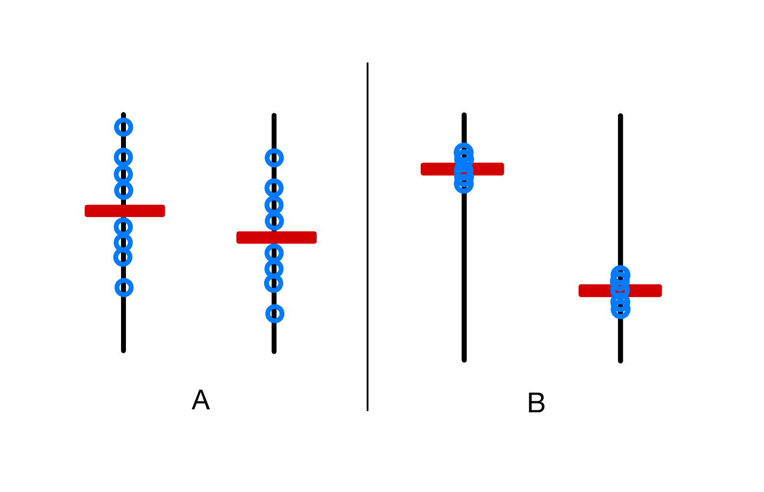
The above figure illustrates the logic behind the F-statistic. Say the red bar is the calculated mean of the data, and the blue dots are scattered data points around the mean.
Between situation A and B, in which situtation does the difference between the two means seem more significant?
It is clear that the difference is more prominent in situation B, because there is more variation between the red bar, and less variation within the blue dots.
This ratio makes their differences seem clear, and this is roughly what the F-statistic is trying to measure.
Hence, if the F-statistic is large, it means the difference between the groups is more significant.
Sum of Squares
The F-statistic is calculated using the sum of squares.
Let us first define the following:
- $k$: number of groups
- $n_j$: number of data points in group $j$
- $n$: sum of $n_j$ for all $j$
- $x_{ij}$: $i$th data point in group $j$
- $\bar{x}_j$: sample mean of group $j$
- $\bar{x}$: mean of all data points (overall mean)
Total Sum of Squares (SS)
Total sum of squares is the sum of squared differences between each data point and the overall mean:
$$ SS_{Total} = \sum_{j=1}^k \sum_{i=1}^{n_j} (x_{ij} - \bar{x})^2 $$
$SS_{Total}$ can be decomposed into two parts:
$$ SS_{Total} = SS_{Between} + SS_{Within} $$
Sum of Squares Between (SSB)
Sum of squares between is the sum of squared differences between each group mean and the overall mean:
$$ \begin{equation*} \label{eq:ssb} \tag{SSB} SS_{Between} = \sum_{j=1}^k \sum_{i=1}^{n_j} (\bar{x}_j - \bar{x})^2 = \sum_{j=1}^k n_j (\bar{x}_j - \bar{x})^2 \end{equation*} $$
Sum of Squares Within (SSW)
Sum of squares within is the sum of squared differences between each data point and its group mean:
$$ \begin{equation*} \label{eq:ssw} \tag{SSW} SS_{Within} = \sum_{j=1}^k \sum_{i=1}^{n_j} (x_{ij} - \bar{x}_j)^2 \end{equation*} $$
This is also known as the residual sum of squares or the error sum of squares.
Mean Square
But we cannot compare the sum of squares directly.
Because the sum becomes larger as the sample size increases, we want to take the sample size into account to make the comparison more meaningful.
We instead use a modified version called mean square, which is the sum of squares divided by the degrees of freedom.
Mean Square Between (MSB)
The degrees of freedom for $\eqref{eq:ssb}$ is $k-1$.
Very roughly, think of this as: the outcome of this formula is already fixed, there’s an overall mean, and we have $k$ group means that affect the overall mean. We are free to choose $k-1$ of the group means, but the last group mean is determined by the rest.
Therefore, the mean square between is:
$$ MSB = \frac{SS_{Between}}{k-1} $$
Mean Square Error (MSE)
The degrees of freedom for $\eqref{eq:ssw}$ is $n-k$.
Again, roughly we are using all $n$ data points, but the $k$ group means are determined by the $n$ data points. So we lose $k$ degrees of freedom.
$$ MSE = \frac{SS_{Within}}{n-k} $$
F-Statistic
The F-value is calculated as follows:
$$ F = \frac{MSB}{MSE} $$
Now we compare this F-value to the F-distribution (with $k-1$ and $n-k$ degrees of freedom) to obtain the p-value.
One-Way ANOVA
Why is it called “one-way”?
It is called “one-way” because this test deals with data with a single factor of influence (predictor variable).
For example, if we wanted to compare the effects of three different fertilizers on plant growth, type of fertilizers will be the single predictor variable and plant height will be the response variable.
Notice that the predictor is categorical.
Each subject (e.g. plant) is allocated to one and only one group (e.g. fertilizer).
Assumptions
One-way ANOVA requires the following assumptions:
- Continuous dependent variable: the dependent variable is continuous (quantitative)
- Categorial independent variable: no overlapping subjects between groups
- No significant outliers: must be accounted for
- Normality: each dependent variable is approximately normal
- Although one-way ANOVA is robust to violations of normality to a certain degree, it is still a good idea to check the normality of the residuals
- Equal variance: each dependent variable has the same variance
F-Test
Given $k$ groups, one-way ANOVA tests the following null hypothesis:
$$ H_0: \mu_1 = \mu_2 = \dots = \mu_k $$
In this case, the alternative hypothesis is:
$$ \text{At least one pair of means are significantly different} $$
When the null hypothesis true, the F-statistic follows the F-distribution with $k-1$ and $n-k$ degrees of freedom.
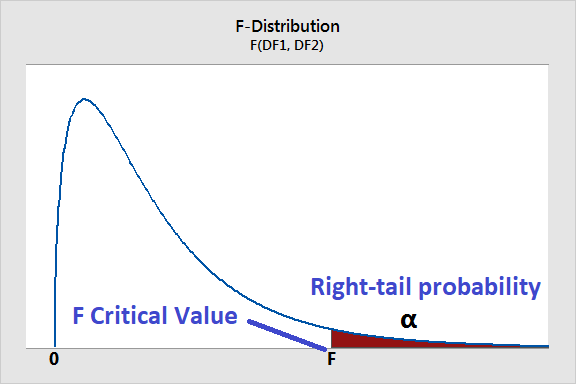
When our null hypothesis is true (the groups are not significantly different), two variations are approximately equal so the F-ratio will be closer to 1.
Hence the peak of the F-distribution is at $\le 1$ (1 ideally, but slightly less than 1 for small degrees of freedom), and being further away to the right means the groups are more significantly different.
We place the F-value on the F-distribution and calculate the p-value.
One-Way ANOVA Summary Table
Typically, we use the following table to summarize the results of ANOVA:
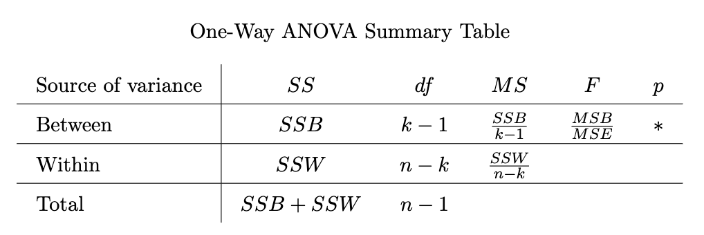
These results from ANOVA are often reused in post-hoc tests.
Two-Way ANOVA
To be added
Why is it called “two-way”?
It is called “two-way” because this test deals with data with two factors of influence (predictor variables).
For example, if we wanted to compare the effects of three different fertilizers and two different types of soil on plant growth, type of fertilizers and type of soil will be the predictor variables, and plant height will be the response variable.
Assumptions
Same as one-way ANOVA.