Post-Hoc Test
As the name suggests, post-hoc test is performed after a test to correct error rates and assess the significance of the results.
Table of contents
Error Rates in Multiple Comparison
Suppose we are testing a family of $m$ hypotheses.
Let’s denote:
| $H_0$ is true | $H_A$ is true | ||
|---|---|---|---|
| Test declared insignificant | $U$ | $T$ | $m - R$ |
| Test declared significant | $V$ | $S$ | $R$ |
| $m_0$ | $m - m_0$ | $m$ |
where each cell represents the number of hypotheses:
- $m_0$: the number of true null hypotheses
- $R$: the number of rejected null hypotheses
- $U$: the number of true negatives
- $T$: the number of false negatives
- $V$: the number of false positives
- $S$: the number of true positives
Family-Wise Error Rate
Family-wise error rate (FWER) is the probability of making at least one Type I error in a family of tests.
$$ \text{FWER} = P(\text{at least one Type I error}) = P(V \geq 1) $$
False Discovery Rate
False discovery rate (FDR) is the expected proportion of false positives among all rejected hypotheses.
Simply:
$$ \text{FDR} = E\left[\frac{V}{R}\right] $$
What if R = 0?
Formally,
$$ \text{FDR} = E\left[\frac{V}{R} \mid R > 0\right] \cdot P(R > 0) $$
Positive False Discovery Rate
To be added
Bonferroni Correction
As we’ve seen in the multiple comparisons problem, repeating the a pairwise test multiple times increases the FWER.
The Bonferroni correction is a method to correct the FWER to $\alpha$ by rejecting the null hypothesis less frequently in each test.
The idea is simple, which is to correct each significance level to:
$$ \alpha' = \frac{\alpha}{m} $$
where $m$ is the number of pairwise tests.
Bonferroni correction has pros:
- It is simple
- It can be used in any test that produces a p-value
Issues with Bonferroni Correction
The problem with the Bonferroni correction is that it is too conservative.
Although it corrects the FWER to approximately $\alpha$, the power of each test is reduced significantly as the number of tests increases.
Suppose we have $\alpha = 0.05$ and we perform 10 pairwise tests.
Then our Bonferroni-corrected $\alpha’$ for each test is 0.005, and this gets worse as the number of tests increases.
It gets harder and harder to call any result significant.
Holm’s Method
Just like Bonferroni, Holm’s method tries to correct the Type I error rate by controlling the FWER.
Procedure
Let’s say we have $m$ hypotheses to test.
Notice the difference in notation between $p_i$ and $p_{(j)}$.
$p_i$ is the p-value of $H_i$, while $p_{(j)}$ is the $j$-th smallest p-value among $p_i$.
- Calculate the p-value $p_i$ for each test ($1 \leq i \leq m$)
- Sort the p-values in ascending order: $p_{(1)} \leq p_{(2)} \leq \dots \leq p_{(m)}$
- Calculate lowerbound rank $L$:
$$ L = \min\left\{j \in \{1, \dots, m\} \mid p_{(j)} > \frac{\alpha}{m + 1 - j}\right\} $$
- Reject all null hypotheses with $p_i < p_{(L)}$
Alternatively
- Calculate the p-value $p_i$ for each test ($1 \leq i \leq m$)
- Sort the p-values in ascending order: $p_{(1)} \leq p_{(2)} \leq \dots \leq p_{(m)}$
- Reject all $p_{(j)}$ such that
$$ p_{(j)} < \frac{\alpha}{m + 1 - j} $$
Comparison to Bonferroni
Both Bonferroni and Holm’s method control the FWER to $\alpha$.
However Holm’s method is at least as powerful as Bonferroni correction, and thus less conservative.
Anything Bonferroni rejects, Holm’s method will also reject.
Proof
Suppose Bonferroni rejects $H_{0i}$ for some $i \in [1, m]$. Then $p_i < \frac{\alpha}{m}$.
Because
We have $p_i < \frac{\alpha}{m + 1 - L} < p_{(L)}$ by definition.
So Holm’s method will also reject $H_{0i}$.
q-Value
Remember that running multiple tests suffers increased overall Type I error. So we use correction methods on the p-value to stabilize the FWER.
However, controlling the FWER to correct type I error often becomes too conservative.
So we look for other methods to correct Type I errors.
Instead of trying to control the FWER, we can try to control the false discovery rate (FDR), and use a q-value which is the FDR analogue of the p-value.
For a recap, the FDR is the expected proportion of false positives among all rejected null hypotheses.
So compared to FWER which measures the chance of making any false positives, FDR is more lenient.
The q-value of a test is the minimum FDR at which the test may be called significant.
Benjamini-Hochberg Procedure
Benjamini-Hochberg procedure is a method to control the FDR.
If we set a threshold $q$ and follow the procedure, $\text{FDR} \leq q$.
Procedure
- Calculate the p-value $p_i$ for each test ($1 \leq i \leq m$)
- Sort the p-values in ascending order: $p_{(1)} \leq p_{(2)} \leq \dots \leq p_{(m)}$
- Calculate the rank $L$
$$ \begin{equation*} \label{eq:bh_rank} \tag{Maximum Rank} L = \max\left\{j \in \{1, \dots, m\} \mid p_{(j)} < \frac{q}{m}\cdot j\right\} \end{equation*} $$
- Reject all null hypotheses with $p_i < p_{(L)}$.
Comparison to controlling FWER
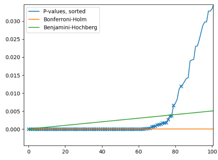
The slope of Benjamini-Hochberge threshold is defined by $q/m$ (see \ref{eq:bh_rank}).
The p-values below each line are the rejected ones (discoveries).
From the graph, we see that Benjamini-Hochberg procedure makes more discoveries than well-known methods that control FWER.
Tukey’s HSD Test
HSD stands for honestly significant difference, which is the minimum difference between two means that is considered (actually/honestly) statistically significant.
So Tukey’s HSD test is a method that calculates the HSD, and checks which pair has a significant difference (i.e. greater than HSD).
It works better than the Bonferroni correction in that it maintains the FWER at $\alpha$ but without losing as much power.
Typically, Tukey’s HSD test is used after ANOVA. However, it can be used standalone as well.
The null hypothesis of Tukey’s HSD test is:
$$ H_0: \forall i, j \in [1, k],\; \mu_i = \mu_j $$
Assumptions
Tukey’s test assumes the following:
- The observations are independent (within and among)
- Each group follows a normal distribution
- Homogeneity of variance in each group
- The sample sizes are equal ($n_k = n$)
If the sample sizes are unequal, Tukey's test becomes more conservative.
Studentized Range Distribution
Suppose we have $k$ populations with normal distribution, and we each take a sample of size $n$.
Let $\bar{x}_{min}$ and $\bar{x}_{max}$ be the smallest and largest sample means respectively, and $s_p$ the pooled standard deviation (with equal sample sizes).
The following random variable has a Studentized range distribution:
$$ Q = \frac{\bar{x}_{max} - \bar{x}_{min}}{s_p / \sqrt{n}} $$
Largest difference between two sample means measured by the standard error.
HSD
Test Statistic
We use the following statistic to measure the difference in means:
$$ \frac{\mid\bar{x}_i - \bar{x}_j\mid}{\sqrt{MSE / n}} $$
where $\bar{x}_i$ and $\bar{x}_j$ are the sample means of group $i$ and $j$ respectively.
When null hypothesis is true, the statistic follows the studentized range distribution.
Critical Value of Studentized Range Distribution
We denote the critical value as
$$ q_{\alpha, \nu, k} $$
where:
- $\alpha$ is the significance level
- $\nu$ is the degrees of freedom of the distribution
- $k$ is the number of groups
We then compare our statistic to a critical value of the distribution. If the statistic is greater than the critical value, we reject the null hypothesis.
The Studentized range distribution is measured on the largest difference, so it makes sense that any difference measure greater than the critical value should be considered significant.
Just like z-scores and t-scores, the values can be obtained from a table.
Defining HSD
For our differences to be significant, we need the following to be true:
\[\frac{\mid\bar{x}_i - \bar{x}_j\mid}{\sqrt{MSE / n}} \geq q_{\alpha, \nu, k}\]We can rearrange the inequality to get the following:
\[\mid\bar{x}_i - \bar{x}_j\mid \geq q_{\alpha, \nu, k} \cdot \sqrt{\frac{MSE}{n}}\]The right-hand side of the inequality is then defined HSD:
$$ HSD = q_{\alpha, \nu, k} \cdot \sqrt{\frac{MSE}{n}} $$
where:
$q_{\alpha, \nu, N}$ is the critical value of the studentized range distribution with $\alpha$ significance level, $\nu$ degrees of freedom, and $k$ groups
Standard error of the group mean:
- $MSE$ is the mean square errror (or within), which you can get from the ANOVA summary table
- $n$ is the sample size of each group (which is assumed to be all equal)
Dunnett’s Test
To be added
Williams Test
To be added