Classification
When response variable is qualitative or categorical, we perform classification.
Classification could be simply predicting the class of observations:
\[f(x) \in \{C_1, C_2, \ldots, C_K\}\]But more profoundly, it would about estimating the conditional probability that an observation belongs to a certain class.
Classification VS Clustering
The difference between classification and clustering is that clustering is essentially unsupervised learning.
Unlike classification, there is no predefined notion of classes or labels for the observations during clustering.
Table of contents
Bayes Classifier
Bayes classifier or Bayes optimal classifier assigns an observation to the class that maximizes the posterior probability:
$$ k^\ast = \arg\max_k P(Y = k \mid X = x) $$
Given an observation, what is the probability that it belongs to class $k$? If it’s high, then it must belong to that class $k$.
This is a natural and rational way to formulate classification, and we rarely know the true posterior probabilities.
Hence the name “optimal”.
Decision Boundary
Decision boundary is the surface that separates the classes.
Decision boundary between two classes $i$ and $j$ is the set of points $\boldsymbol{x}$ where the posterior probabilities are equal.
For linear classifiers, we would have learned a set of weights/parameters $\hat{\beta}_i$ and $\hat{\beta}_j$ that determine the probability of $\boldsymbol{x}$ belonging to class $i$ and $j$.
Then our decision boundary would be the set of coordinates $\boldsymbol{x} \in \mathbb{R}^p$ such that:
$$ \hat{\beta}_{i0} + \hat{\beta}_i^\top \boldsymbol{x} = \hat{\beta}_{j0} + \hat{\beta}_j^\top \boldsymbol{x} \iff \hat{\beta}_{i0} - \hat{\beta}_{j0} + (\hat{\beta}_i - \hat{\beta}_j)^\top \boldsymbol{x} = 0 $$
For clarity we denote the intercept term separately from the weights here.
Affine Subspace
\[\overbrace{\hat{\beta}_{i0} - \hat{\beta}_{j0}}^a + (\underbrace{\hat{\beta}_i - \hat{\beta}_j}_\boldsymbol{b})^\top \boldsymbol{x} = 0\]The decision boundary,
\[\{\boldsymbol{x} \in \mathbb{R}^p \mid a + \boldsymbol{b}^\top \boldsymbol{x} = 0\}\]Defines a $(p-1)$-dimensional affine subspace in $\mathbb{R}^p$.
Remeber that a one-dimensional affine subspace is a line, and a two-dimensional affine subspace is a plane.
For $K$ classes, there would be a total
\[{K \choose 2} = \frac{K(K-1)}{2}\]decision boundaries.
Why Not Regular Linear Regression?
In the case of binary classification with label $\{0, 1\}$, our regression function
\[f(x) = \E[Y \mid X = x]\]Conveniently becomes the conditional probability:
\[P(Y = 1 \mid X = x)\]Which is what we want for classification.
However, the prediction from linear regression is:
- Hard to interpret as probability: There is no way to bind the prediction to $[0, 1]$.
- Hard to define a threshold or cutoff for classification
- Doomed for multi-class classification
- Mapping qualitative variables to a sequence of numerical labels i.e. $\{1, 2, 3\}$ introduces a sense of order and distance between the classes, when there is none.
Masking Phenomenon
Take a look at the third bullet point above. One of the reasons why linear regression is doomed for multi-class classification is masking.
Masking is a phenomenon where the decision boundary collapses for multi-class classification.
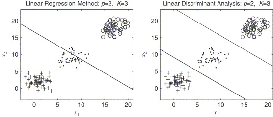
The effect is that some classes are “masked” by others, and an observation is never assigned to the masked class.
This phenomenon becomes more severe as the number of classes increases.
Misclassification Rate
Unlike regression, where we use MSE to measure performance, in classification we use misclassification rate or error rate.
It is simply the proportion of misclassified observations:
$$ \text{Error rate} = \sum_{i=1}^n \frac{I(y_i \neq \hat{y}_i)}{n} $$
Logistic Regression
Discriminant Analysis
Threshold
In the context of binary classification, selecting class $k$ with the highest $p_k(x)$ is equivalent to setting a threshold, say $0.5$, and asking the question:
\[P(Y = 1 \mid X = x) > 0.5\]If yes, then $Y = 1$.
Different thresholds would lead to different misclassification rates, which is our measure of performance in classification.
So we need to find the optimal threshold as well.