Statistical Hypothesis Testing
Table of contents
Different Types of Data Analysis
Confirmatory Data Analysis
Confirmatory data analysis is when the researcher already has a clear hypothesis and tries to test whether the data confirms or rejects it.
For example, a researcher may hypothesize that a new drug is more effective than a placebo.
Then, the researcher would collect data and perform statistical tests to compare the two groups.
This page focuses on confirmatory data analysis.
Exploratory Data Analysis
Exploratory data analysis is when the researcher does not have a clear hypothesis and tries to find patterns or trends in the data.
May be used to generate hypotheses for confirmatory data analysis.
Setting Up a Hypothesis
Say we want to test the effectiveness of a new drug.
Let $A$ be population of blood pressure of people who take the new drug, and $B$ be the population of blood pressure of people who take a placebo.
For the drug to be effective, we want $\mu_A \ne \mu_B$, where $\mu_A$ and $\mu_B$ are the population means of $A$ and $B$.
Notice that the hypothesis is about the population, not the sample.
In hypothesis testing, we set up two hypotheses:
Null Hypothesis
The null hypothesis is the negation of the hypothesis we want to confirm.
With our example, the null hypothesis is:
$$ \begin{equation} \label{eq:null-h} \tag{Null Hypothesis} \mu_A = \mu_B \end{equation} $$
This would mean that the drug is not effective.
Alternative Hypothesis
The alternative hypothesis is the hypothesis we want to confirm.
With our example, the alternative hypothesis is:
$$ \begin{equation} \label{eq:alt-h} \tag{Alternative Hypothesis} \mu_A \ne \mu_B \end{equation} $$
This would mean that the drug is effective.
Proof by Contradiction
Hypothesis testing takes the following approach:
- Set up the null hypothesis and alternative hypothesis
- Assume a distribution where the null hypothesis is true
- Calculate a test statistic from the real sample data
- Test how this statistic fits into this assumed distribution
- If the real data statistic is unlikely when the null hypothesis is true, then we reject the null hypothesis
- By rejecting the null hypothesis, we accept the alternative hypothesis
- Otherwise, we fail to reject the null hypothesis
Notice the wording: fail to reject the null hypothesis. Failing to reject does not equal accepting the null hypothesis or rejecting the alternative hypothesis.
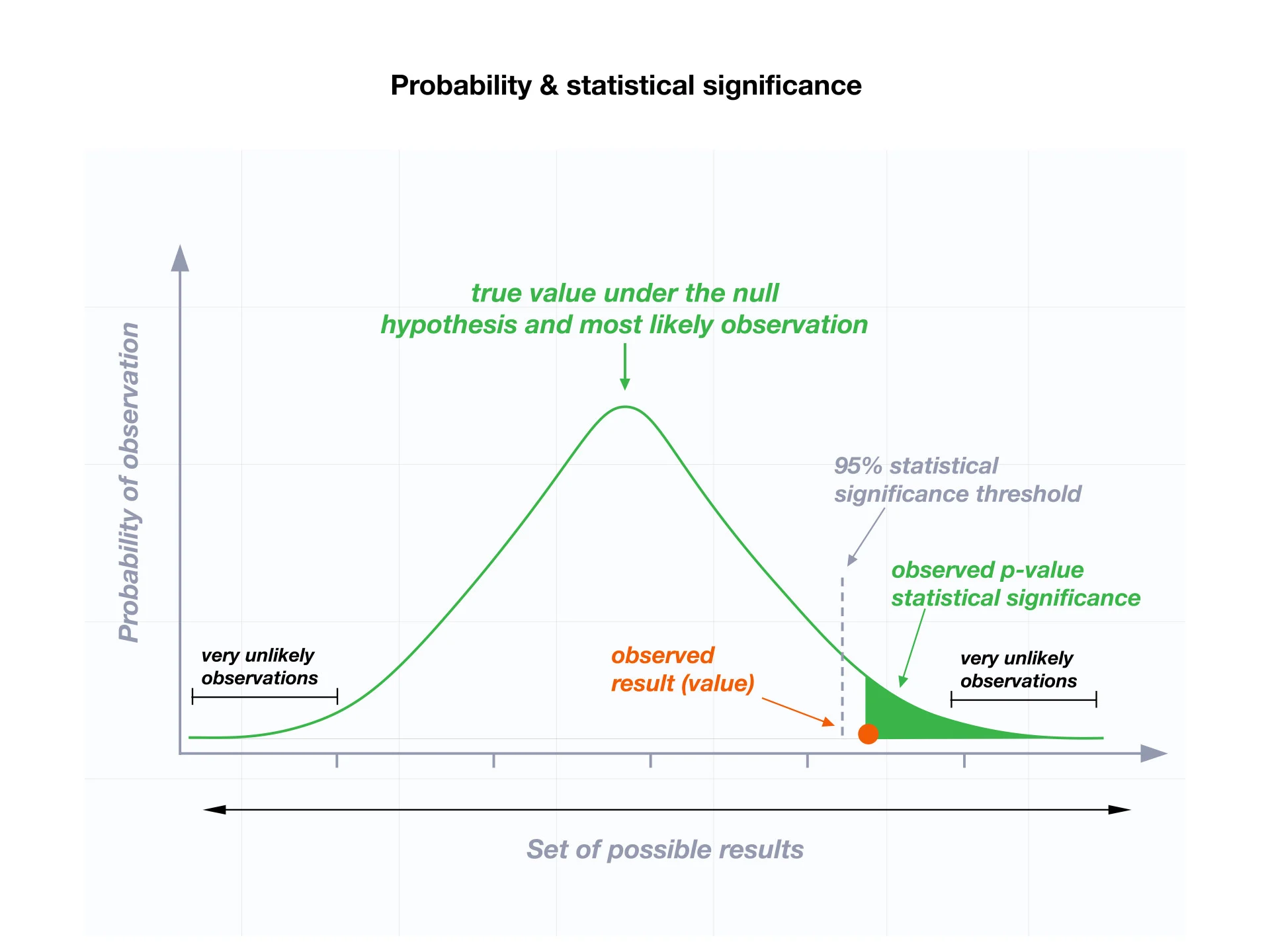
p-Value
The $p$-value is:
The probability of observing the data in a distribution that assumes the null hypothesis is true.
So if the p-value of a real data is low, then the data is unlikely to occur when the null hypothesis is true. Which in turn means that the null hypothesis is unlikely to be true.
So the next question is:
- What is considered a low $p$-value?
Significance Level $\alpha$
Whether we reject the null hypothesis or not depends on the significance level, commonly denoted by $\alpha$.
Most commonly used significance level is $\alpha = 0.05$.
Rejection Region
The rejection region $R$ refers to the area on the left and right tails of the distribution that we would reject the null hypothesis.
More formally
\[R = \{ x \mid T(x) < -c \lor T(x) > c \}\]Where $T(x)$ is the test statistic and $c$ is the critical value.
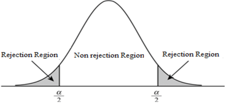
For $\alpha = 0.05$, the rejection region would be on each side of the distribution, 2.5% each.
One-Tailed Test / One-Sided Test
One-tailed test is when we reject the null hypothesis by considering only one tail of the distribution, and thus $\alpha / 2$.
Two-Tailed Test / Two-Sided Test
Two-tailed test is when we reject the null hypothesis by considering both tails of the distribution, and thus the whole $\alpha$.
Unless there is a reason to use one-tailed test, it is much more common to use two-tailed test.
Statistically Significant
If the $p$-value is less than $\alpha$, then the data is statistically significant.
$$ p < \alpha $$
Then we reject the null hypothesis and accept the alternative hypothesis.
Otherwise, we have no grounds to reject the null hypothesis.
Different Methods for Hypothesis Testing
Hypothesis Testing and Confidence Interval
The relationship between confidence interval and hypothesis testing is like a mirror image.
$$ \text{Significance Level}\; \alpha = 1 - \text{Confidence Level} $$
With a 95 CI, we infer a likely (with 95% chance) range of the population statistic based on the sample statistic computed from real data.
Then we test if our null hypothesis fits into this range.
For instance, with our example null hypothesis, we can calculate a 95 CI for $\mu_A - \mu_B$, and see if it contains 0.
If not, then we reject the null hypothesis.
On the other hand, with hypothesis testing, we first assume that the null hypothesis is true, and then calculate a sample statistic from the real data.
Then we test how this sample statistic fits into this assumed null hypothesis.
For instance, with our example null hypothesis, we obtain a distribution of $\mu_A - \mu_B$ of which the mean is 0.
Then we calculate the probability $p$ of observing the real data, and see if it is less than $\alpha = 0.05$.
If so, then we reject the null hypothesis.
Plotting Graphs in Hypothesis Testing
Error Bars
With bar plots and scatter plots, you’ll often see error bars.
It is important to describe in the legends which metric is used for the error bars, because it can mean different things.
Suppose we have a bar plot with sample mean as the variable,
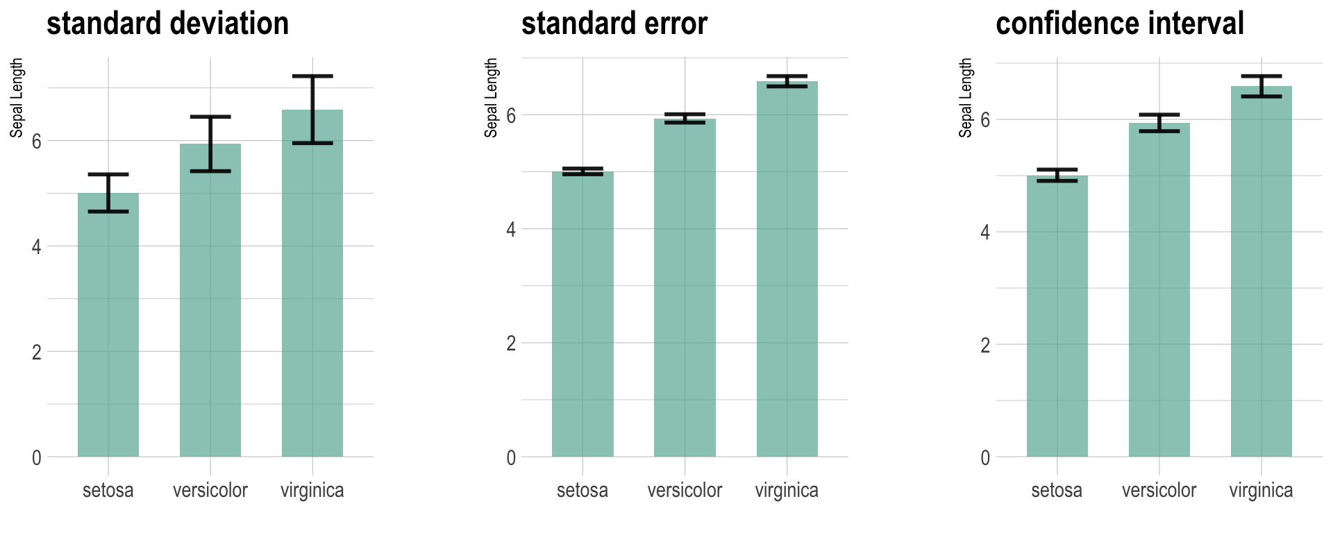
- Standard deviation
- The error bars represent the dispersion of the sample
- Does not represent a probability
- Standard error of the mean
- The error bars represent the probability of the sample mean
- Confidence interval
Indicating Statistical Significance
In figures and charts, we commonly use asterisks ($*$) to indicate statistical significance.
Although the figure below does not, make sure to indicate what the asterisks mean in the legends.
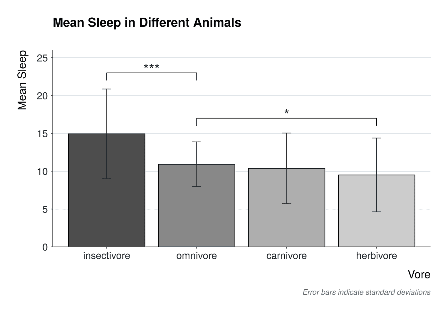
Commonly used symbols are:
- $p < 0.05$: $*$
- $p < 0.01$: $**$
- $p < 0.001$: $***$
- Non-significant: $\text{N.S.}$